Dynamic Sensor Scheduling for Thermal Management in Biological Wireless Sensor Networks

Abstract

Biological sensors are a very promising technology that will take healthcare to the next level. However, there are obstacles that must be overcome before the full potential of this technology can be realized. One such obstacle is that the heat generated by biological sensors implanted into a human body might damage the tissues around them. Dynamic sensor scheduling is one way to manage and evenly distribute the generated heat. In this paper, the dynamic sensor scheduling problem is formulated as a Markov decision process (MDP). Unlike previous works, the temperature increase in the tissues caused by the generated heat is incorporated into the model. The solution of the model gives an optimal policy that when executed will result in the maximum possible network lifetime under a constraint on the maximum temperature level tolerable by the patient's body. In order to obtain the optimal policy in a lesser amount of time, two specific types of states are aggregated to produce a considerably smaller MDP model equivalent to the original one. Numerical and simulation results are presented to show the validity of the model and superiority of the optimal policy produced by it when compared with two policies one of which is specifically designed for biological wireless sensor networks.

1. Introduction

Biological wireless sensor networks (BWSNs) are networks made up of biological sensors (biosensors, for short) which are tiny wireless devices attached or implanted into the body of a human or animal to monitor and control biological processes. They have originated because of the need to improve and modernize healthcare. The sensing elements in biosensors are biological materials such as enzymes and antibodies. They are integrated into transducers for producing electrical signals in response to biological reactions and changes.

A famous application of BWSNs is the geodesic sensor network developed by EGI corporation [1]. In this application, a cap-based system of electrodes is worn by a patient for continuous brain monitoring. Figure 1 shows a girl wearing a geodesic sensor network. The sensor network collects electroencephalographical (EEG) measurements of the brain and delivers them to a controller which processes them and displays the results. Another example is glucose biosensors which monitor the blood glucose level in a diabetic patient. They can be used to optimally control the infusion of insulin into the patient or to initiate a prompt medical intervention. An example of glucose biosensors can be found in [2].

Figure 1

A girl wearing a geodesic sensor network [1].

In addition to being energy-constrained, biosensors are also temperature-constrained. This is due to the heat generated as a result of their operation in temperature-sensitive environments like the human body. Radiation which is mainly due to wireless communication is the major source of heat. (Another major source of heat is the radiation due to RF recharging in rechargeable BWSNs. This source of heat is not considered here since we are assuming nonrechargeable biosensors.) The tissues surrounding biosensors absorb the RF energy which gets transformed into heat. This effect is balanced by the human thermoregulatory system. However, if the generated heat is larger than what can be drained, the temperature of the tissues rises. If the blood flow is not sufficient, the affected tissues might be damaged.

Thermal effects caused by biosensors are a major obstacle in the road to realizing the full vision for BWSNs. These effects can be mitigated through the use of effective thermal management techniques. One such technique is the dynamic scheduling of the transmission of biosensor measurements. As will be shown, this technique is very effective in reducing the temperature rise in the tissues due to heating. In this paper, the thermal management problem in BWSNs is studied. It is shown how it can be modeled as a stochastic control problem. Randomness is present due to the random behavior of the wireless channel between biosensors and the base station where measurements are collected and processed.

Toward that end, the framework of MDPs is used to build a mathematical model of the BWSNs under study. The model is then solved to obtain a policy which dictates how the BWSN should be operated in order to avoid a hazardous temperature increase. The obtained policy can achieve the best balance between transmission energy consumption and temperature increase. It also results in the minimum temperature increase when compared to existing policies.

In order to reduce the size of the MDP model, state aggregation is used. Two classes of system states are identified. A considerable reduction in the size of the MDP model is achieved when the states in these two classes are aggregated. The equivalence of the reduced MDP model to the original one is established and the reduction in model size is shown. A reduction of as high as 79% can be achieved.

The remainder of the paper is organized as follows. First, the necessary background information is given. Second, the available literature is briefly reviewed. Third, the system under study is described. Then, its MDP model is presented. After that, the minimization of the size of the MDP model using state aggregation is discussed. Then, numerical and simulation results are presented within the context of an example to illustrate the viability of the MDP model. Finally, conclusions and directions for further research are given.

2. Background

This section presents the necessary information to understand how temperature increase is calculated. It also briefly explains MDPs and points out some approaches for handling their state explosion problem.

2.1. Calculating Temperature Increase

RF signals used for wireless communication and recharge of implanted biosensors produce electrical and magnetic fields. When a human gets exposed to electromagnetic fields, the absorbed radiation gets converted into heat which manifests itself as a temperature increase inside the tissues. This phenomenon is balanced by the human thermoregulatory system. If the generated heat is larger than what can be drained, the temperature of the tissues will rise. The tissues might be damaged if the generated heat cannot be regulated by the blood circulation system.

The level of radiation absorbed by the human body when exposed to RF radiation is measured by the specific absorption rate (SAR) which is expressed in units of watts per kilogram (W/Kg). SAR records the rate at which radiation energy is absorbed per unit mass of tissue [3]. SAR is a point quantity. That is, its value varies from one location to another. SAR in the near field (i.e., the space around the antenna of the biosensor) causes the heating of the tissue surrounding the biosensor. It is a function of the current provided to the antenna of the biosensor. As an example to appreciate the importance of this measure, it was reported in [4] that an exposure to an SAR of 8 W/Kg in any gram of tissue in the head for 15 minutes may result in tissue damage.

The Pennes's bioheat equation [5] is the standard for calculating the temperature increase in the body due to heating. This equation can be transformed into a discrete form by using the finite-difference time-domain (FDTD) method [6]. Basically, the area under consideration is divided into cells and the temperature is evaluated in a grid of points defined at the centers of the cells. It is assumed that the temperature of the surrounding cell points is the normal body temperature (i.e., 37°C).

2.2. Markov Decision Processes

An MDP is a model of a dynamic system whose behavior varies with time. The elements of an MDP model are the following [7]:

• (1)

system states,

(2)

possible actions at each system state,

(3)

a reward or cost associated with each possible state-action pair,

(4)

next state transition probabilities for each possible state-action pair.

The solution of an MDP model (referred to as a policy) gives a rule for choosing an action at each possible system state. If the policy chooses an action at time t depending only on the state of the system at time t, it is referred to as a stationary policy. An optimal stationary policy exists over the class of all policies if every stationary policy gives rise to an irreducible Markov chain. This means that one can limit the attention to the class of stationary policies.

An interesting class of MDPs is the class of MDPs with a terminating state. This state is reached with probability one in a finite number of steps. The number of steps represents the lifetime of the Markovian process induced by the MDP model (hence, the lifetime of the modeled system). The solution of the model is a policy which drives the system into the terminating state while optimizing an objective function which may include the lifetime of the system as a parameter.

In order to obtain a policy from an MDP model, it is necessary to form and solve the so-called optimality equation (or Bellman equation). The following is the standard form of this equation with the maximization operator [8]:

$$\begin{array}{cc}& V_n\left(s\right)=\underset{a\in A\left(s\right)}{\max }\left[f\left(s,a\right)+\sum _{s^{\prime }\in S}‍\mathbb{P}\left(s,s^{\prime },a\right)V_{n-\mathrm{1}}\left(s^{\prime }\right)\right],\end{array}$$

(1)

where n is the iteration index, S is the set of system states ( $s\in S$ ), $A(s)$ is the set of actions possible when the system is at state s, $f(s,a)$ is the reward/cost per step, ℙ is the system state transition probability matrix, and $V(s)$ is the optimal value of the objective function when the system is started at state s and the optimal policy is followed.

Equation (1) can be solved using the classical policy iteration, value iteration, and relative value iteration algorithms [8]. However, these algorithms become impractical when the number of system states is large. In such situations, one typically resorts to approximate techniques such as in [9–12]. Another solution for the problem of state explosion is state aggregation [13–17]. In this technique, using some notion of equivalence, equivalent states are combined into one class which is represented by a single state in the reduced MDP model. The new MDP model is equivalent to the original one but with significantly fewer states. In this paper, this technique is used to aggregate two kinds of system states.

3. Related Work

The research on the possible biological effects caused by biosensors and how to mitigate those effects is very recent. Most of the existing research deals with other technical issues such as energy efficiency and quality of service. In this section, we briefly review the limited available literature.

The effect of leadership rotation on a cluster-based biological WSN was studied in [18]. It was observed that rotating the role of which node collects measurements from other sensors and delivers them to the base station can significantly reduce the temperature increase in tissues due to wireless communication. The computation of an optimal rotation sequence involves using the Pennes's bioheat equation [5] and the finite-difference time-domain (FDTD) method [6] to calculate the temperature increase due to a sequence. Because of its time requirement, the authors proposed another scheme to calculate the temperature increase. It is referred to as the temperature increase potential (TIP). It efficiently estimates the temperature increase of a sequence. Using this scheme and a genetic algorithm, they were able to find the minimum temperature increase rotation sequence. They, however, did not consider the effect of the wireless channel and limited energy.

The issue of routing in biological WSNs was studied in [19]. The authors proposed a thermal-aware routing protocol that routes the data away from high temperature areas referred to as hot spots. The location of a biosensor becomes a hot spot if the temperature of the biosensor exceeds a predefined threshold. The proposed protocol achieves a better balance of temperature increase and shows the capability of load balance.

In [20], the sensor scheduling problem is formulated as an MDP. The objective is to find an operating policy that maximizes the network lifetime. The state of a sensor is characterized by its current energy level only. Three kinds of channel state information are considered: global, channel statistics, and local. Considering only the energy level at each sensor gives rise to an acyclic (i.e., loop-free) transition graph which enables the MDP model to converge in one iteration. On the other hand, if the temperature of each sensor is included in the model, the transition graph of the underlying MDP becomes cyclic. This is because when the sensor cools down (i.e., its temperature decreases), it transitions back to a less hot state. An MDP model whose transition graph is cyclic needs more time to converge.

Dynamic sensor activation in networks of rechargeable sensors is considered in [21]. The objective is to find an activation policy that maximizes the event detection probability under the constraint of slow rate of recharge of the sensor. The state of the system is characterized by the energy level of the sensor and whether or not an event would occur in the next time slot. The recharge event is random and recharges the sensor with a constant charge. The model does not include the state of the wireless channel which is very crucial when temperature is considered.

Body sensor networks [22] with energy harvesting capabilities are another kind of WSNs in which each sensor has an energy harvesting device that collects energy from ambient sources such as vibration, light, and heat. In this way, the more costly recharging method which uses radiation is avoided. The interaction between the battery recharge process and transmission with different energy levels is studied in [23]. The proposed policies utilize the sensor's knowledge of its current energy level and the state of the processes governing the generation of data and battery recharge to select the appropriate transmission mode for a given state of the network.

4. System Model

Figure 2 shows a BWSN consisting of three biosensors implanted into the body of a patient. The biosensors communicate with an access point (or base station) over a wireless channel. The wireless access point initiates the data collection process by determining which biosensor is going to transmit the next measurement. A biosensor is selected for transmission based on the current network state and some policies. The wireless access point is assumed to know the global channel state information (CSI) of the wireless channel and the state of each biosensor at each point in time. It is assumed that the instantaneous received signal-to-noise ratio (SNR) fully characterizes the state of the wireless channel.

Figure 2

A patient with three biosensors implanted into his body.

The setup in Figure 2 can mathematically be modeled as a discrete-state system which evolves in discrete time. Thus, the time axis is divided into slots of equal duration $\mathrm{\Delta }T$ and time $t\in {\mathbb{Z}}^{+}$ is the time interval $[t\mathrm{\Delta }T,(t+\mathrm{1})\mathrm{\Delta }T)$ . The state of the system represents its condition at the beginning of a time slot. Control (i.e., which biosensor to choose next) can only be exercised at the beginning of a time slot and not at any other time during the slot. For example, the current temperature and remaining energy of each biosensor and the CSI of the wireless channel are used to represent the state of the system in Figure 2. Also, the number of biosensors is used to represent the number of possible control actions that can be used to control the evolution of the system.

The system in Figure 2 works as follows. At the beginning of each time slot, a biosensor is selected by the base station to transmit its measurement. As a result, the energy and temperature of the selected biosensor change according to its transmission energy requirement which is determined by the state of the wireless channel. Also, the temperature of the neighbors of the selected biosensor increases based on the amount of energy used in the transmission. On the other hand, the temperature of the nonneighboring biosensors decreases. The change in the temperature of the biosensors can be calculated using the Pennes's bioheat equation and the FDTD method (for more details, see Section 2.1.). However, due to the large simulation time required before the temperature change reaches a steady state, this approach is not followed here. Instead, the temperature decrease is assumed to be a constant reduction which occurs whenever the biosensor is not transmitting and not a neighbor of a transmitting biosensor. The temperature increase is also assumed to be directly proportional to the energy consumed by the transmitting biosensor.

Clearly, from the previous description, the location of a biosensor represents a critical point since it experiences the maximum temperature increase. This is because the tissues surrounding a biosensor might be heated continuously due to the local radiation generated by the biosensor itself and the radiation generated by its neighbors.

Let χ be the set of biosensors which have been surgically implanted in the body of a patient and at known locations. Also, let ${{\rm Y}}_i$ be the set of biosensors which are neighbors to biosensor i. Different criteria can be used to compute this set. In this work, the Euclidean distance between biosensors is used. Each biosensor $i\in \chi$ has a battery with an initial energy of ${ℰ}_{\mathrm{0}}$ and a maximum safe temperature level τ which must not be exceeded. In each time slot t, the state of a biosensor i is characterized by two variables which are the current temperature $T_t(i)$ and remaining energy $E_t(i)$ . The energy required for a biosensor i to successfully transmit its measurement to the base station is determined by the state of the wireless channel in time slot t in which it is scheduled. This transmission energy is a random variable that is denoted by $W_t(i)$ and is IID over all sensors and time slots. Due to hardware and power limitations, $W_t(i)$ is discretely distributed over a finite set $\{ϵ,{ϵ}_{\mathrm{2}},\dots ,{ϵ}_L\}$ , where $\mathrm{0}<{ϵ}_{\mathrm{1}}<{ϵ}_{\mathrm{2}}<\cdots <{ϵ}_L<\infty$ and ${ϵ}_j$ is the energy consumed by a biosensor in transmitting its measurement at the jth power level.

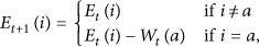
At the end of each time slot, the energy level at each biosensor i is given by the following equation:

$$\begin{array}{cc}& E_{t+\mathrm{1}}\left(i\right)=\{\begin{array}{cc}{E}_t\left(i\right)\hfill & \text{if}\mathrm{\hspace{0.17em}\hspace{0.17em}}i\ne a\hfill \\ E_t\left(i\right)-W_t\left(a\right)\hfill & \text{if}\mathrm{\hspace{0.17em}\hspace{0.17em}}i=a,\hfill \end{array}\end{array}$$

(2)

where a is the index of the sensor selected for transmission. Similarly, the temperature of each biosensor i is given by the following equation:

$$\begin{array}{cc}& T_{t+\mathrm{1}}\left(i\right)=\{\begin{array}{cc}ℱ\left(T_t\left(i\right),W_t\left(a\right)\right)\hfill & \text{if}\mathrm{\hspace{0.17em}\hspace{0.17em}}i=a\mid i\in {{\rm Y}}_a\hfill \\ T_t\left(i\right)-\kappa \hfill & \text{if}\mathrm{\hspace{0.17em}\hspace{0.17em}}i\ne a\mathrm{\hspace{0.17em}\hspace{0.17em}}\&\mathrm{\hspace{0.17em}\hspace{0.17em}}i\notin {{\rm Y}}_a,\hfill \end{array}\end{array}$$

(3)

where ℱ is a function of the transmission power and current temperature of the sensor scheduled for transmission and κ is the amount by which the temperature of a nonneighboring sensor decreases. The symbol ∣ denotes the logical OR operator. It should be noted that the change in temperature experienced by the scheduled biosensor and its neighbors is assumed to be the same. This is a realistic assumption since biosensors in the same neighborhood experience the same amount of radiation.

Finally, the communication between the biosensor and base station occurs over a Rayleigh fading channel with additive Gaussian noise. Hence, the instantaneous received SNR denoted by γ is exponentially distributed with the following probability density function [24]:

$$\begin{array}{cc}& P\left(\gamma \right)=\frac{\mathrm{1}}{{\gamma }_{\mathrm{0}}}\exp \left(-\frac{\gamma }{{\gamma }_{\mathrm{0}}}\right),\end{array}$$

(4)

where ${\gamma }_{\mathrm{0}}$ is the average received SNR.

Such a wireless channel can be modeled as a finite-state Markov chain (FSMC) [25, 26]. The model can be built as follows. For a wireless channel with K states, the state boundaries (i.e, SNR thresholds) are denoted by ${\mathrm{\Gamma }}_{\mathrm{1}},{\mathrm{\Gamma }}_{\mathrm{2}},\dots ,{\mathrm{\Gamma }}_K,{\mathrm{\Gamma }}_{K+\mathrm{1}}$ where ${\mathrm{\Gamma }}_{\mathrm{1}}=\mathrm{0}$ and ${\mathrm{\Gamma }}_{K+\mathrm{1}}=\infty$ . The channel is said to be in state $s_i$ if the SNR is between ${\mathrm{\Gamma }}_i$ and ${\mathrm{\Gamma }}_{i+\mathrm{1}}$ where $i=\mathrm{1,2},\dots ,K$ . It is assumed that the SNR remains the same during packet transmission and only transitions to the current or adjacent states are allowed.

The steady-state probability of the ith state of the FSMC is given by

$$\begin{array}{cc}& P\left(s_i\right)=\exp \left(-\frac{{\mathrm{\Gamma }}_i}{{\gamma }_{\mathrm{0}}}\right)-\exp \left(-\frac{{\mathrm{\Gamma }}_{i+\mathrm{1}}}{{\gamma }_{\mathrm{0}}}\right)\end{array}$$

(5)

and thus the state transition probabilities are

$$\begin{array}{cc}& P\left(s_{i+\mathrm{1}}\mid s_i\right)\approx \frac{N\left({\mathrm{\Gamma }}_{i+\mathrm{1}}\right)\mathrm{\Delta }t}{P\left(s_i\right)},\\ P\left(s_{i-\mathrm{1}}\mid s_i\right)\approx \frac{N\left({\mathrm{\Gamma }}_i\right)\mathrm{\Delta }t}{P\left(s_i\right)},\end{array}$$

(6)

where $N({\mathrm{\Gamma }}_i)$ is the average number of times per unit interval that the SNR crosses level ${\mathrm{\Gamma }}_i$ and $\mathrm{\Delta }t$ is the packet duration. $N({\mathrm{\Gamma }}_i)$ can be computed using the following equation [27]:

$$\begin{array}{cc}& N\left({\mathrm{\Gamma }}_i\right)=\sqrt{\mathrm{2}\pi {\mathrm{\Gamma }}_i}{f}_d{e}^{-{\mathrm{\Gamma }}_i},\end{array}$$

(7)

where $f_d$ is the maximum Doppler frequency defined as $f_d=v/\lambda$ with v being the speed of the subject and λ being the wavelength.

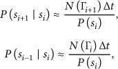
Therefore, the transmission energy requirement for a biosensor i follows a Markov chain with L states and transition probabilities $P[W_{t+\mathrm{1}}(i)=w^{\prime }\mid W_t(i)=w]$ , where $w,w^{\prime }\in \{{ϵ}_j{\}}_{j=\mathrm{1}}^L$ . This channel model has been verified to be precise when the fading process is slow [25] such as in biosensor applications.

5. MDP Model

5.1. Formulation

The purpose of the MDP formulation of the system described in the previous section is to find a policy π that prescribes the best action to take in each state of the system so as to maximize the long-term expected lifetime of the system. The policy π is a stationary policy which means that it is independent of time and depends only on the state of the system. Next, we give the details of the MDP model.

5.1.1. State Set

The state of the system with $|\Pi |$ biosensors at time t is described by a $(\mathrm{3}\times |\Pi |)$ -dimensional vector. That is,

$$\begin{array}{l}{s}_t=\{\left(T_t\left(\mathrm{1}\right),E_t\left(\mathrm{1}\right),W_t\left(\mathrm{1}\right)\right),\left(T_t\left(\mathrm{2}\right),E_t\left(\mathrm{2}\right),W_t\left(\mathrm{2}\right)\right),\dots ,\\ \hspace{1em}\hspace{1em}\phantom{\text{=}}\left(T_t\left(\left|\Pi \right|\right),E_t\left(\left|\Pi \right|\right),W_t\left(\left|\Pi \right|\right)\right)\}.\end{array}$$

(8)

Let S be the set of possible system states. Then, the number of possible system states is $|S|=|T{|}^{|\Pi |}\times |E{|}^{|\Pi |}\times |W{|}^{|\Pi |}$ , where $|T|$ , $|E|$ , and $|W|$ are the numbers of possible temperatures, residual energies, and transmission energy levels, respectively.

The system enters a terminating state when any one of the following two conditions is true:

• (1)

temperature of any biosensor is harmful (i.e., $T_t(i)\ge \tau$ , where τ is a maximum threshold on the allowed temperature increase);

(2)

a biosensor cannot transmit its measurement due to lack of enough energy (i.e., $E_t(i)<W_t(i)$ ) (this condition also accounts for the case when $E_t(i)=\mathrm{0}$ ).

Once the system is in a terminating state, the system must be halted to protect the patient. The system can then be restored to an initial state by recharging the biosensors and letting them cool down.

5.1.2. Action Set

In each time slot, based on the current state of the system, the base station chooses an action (i.e., a biosensor to transmit its measurement). The set of possible actions consists of the indexes of all biosensors. In other words, the set of actions available in each state $s\in S$ is $A(s)=\{\mathrm{1,2},\dots ,|\Pi |\}$ .

5.1.3. Reward Function

Let $R(s,a)$ be the instantaneous reward earned by the network due to action $a\in A(s)$ when the system is in state $s\in S$ . Since the goal is to maximize the expected network lifetime, the reward function can be defined as

$$\begin{array}{cc}& R\left(s,a\right)=\mathrm{1}\end{array}$$

(9)

which assigns a unit reward to each time slot as long as the network is in a nonterminating state. Therefore, the expected sum of rewards obtained before the network reaches a terminating state represents the network lifetime. It should be pointed out that the expectation is taken over all possible state sequences generated by a given policy.

5.1.4. Transition Probability Function

The behavior of the system is described by $|A|$    $|S|\times |S|$ transition probability matrices. Each matrix is denoted by ${\mathbb{P}}_{s_t,s_{t+\mathrm{1}}}(a)$ which is the probability that choosing an action a when in state $s_t$ will lead to state $s_{t+\mathrm{1}}$ . More formally, ${\mathbb{P}}_{s_t,s_{t+\mathrm{1}}}(a)$ can be rewritten as follows:

$$\begin{array}{l}\mathbb{P}\left[s_{t+\mathrm{1}}\mid s_t,a=k\right]=\prod _{i\in \Pi }\{P\left[T_{t+\mathrm{1}}\left(i\right)\mid T_t\left(i\right),W_t\left(i\right),a=k\right]\\ \hspace{1em}\hspace{1em}\hspace{1em}\hspace{1em}\hspace{1em}\hspace{1em}\hspace{1em}\hspace{1em}\hspace{1em}\hspace{0.17em}\phantom{=.}\times P\left[E_{t+\mathrm{1}}\left(i\right)\mid E_t\left(i\right),W_t\left(i\right),a=k\right]\\ \hspace{1em}\hspace{1em}\hspace{1em}\hspace{1em}\hspace{1em}\hspace{1em}\hspace{1em}\hspace{1em}\hspace{1em}\hspace{0.17em}\phantom{=.}\times \hspace{0.17em}\hspace{0.17em}P\left[W_{t+\mathrm{1}}\left(i\right)\mid W_t\left(i\right)\right]\}.\end{array}$$

(10)

5.1.5. Value Function

The thermal management problem is formulated as an infinite-horizon MDP using the average reward criterion [7]. So, let $V_{\pi }(s_{\mathrm{0}})$ be the expected network lifetime given that the policy π is used with an initial state $s_{\mathrm{0}}$ . Then, the maximum expected network lifetime $V^{*}(s_{\mathrm{0}})$ starting from state $s_{\mathrm{0}}$ is given by

$$\begin{array}{cc}& V^{*}\left(s_{\mathrm{0}}\right)=\underset{\pi }{\max }\hspace{0.17em}{V}_{\pi }\left(s_{\mathrm{0}}\right).\end{array}$$

(11)

The optimal policy ${\pi }^{*}$ is the one that achieves the maximum expected network lifetime at all nonterminating states. Hence, it gives the optimal sensor transmission schedule.

The relative value iteration (RVI) algorithm [8] is used to numerically solve the following recursive equation for $n>\mathrm{0}$ :

$$\begin{array}{cc}& V_n\left(s\right)=\underset{a\in A\left(s\right)}{\max }\left[R\left(s,a\right)+\sum _{s_{t+\mathrm{1}}\in S}\mathbb{P}\left(s_t,s_{t+\mathrm{1}},a\right)V_{n-\mathrm{1}}\left(s_{t+\mathrm{1}}\right)\right].\end{array}$$

(12)

In (12), the subscript n denotes the iteration index. As $n\to \infty$ , $V_n\to V^{*}$ .

5.2. Minimizing the Size of the MDP Model through State Aggregation

The large state space of the MDP model makes the computation of the optimal policy a highly intensive process and thus only feasible for small-scale networks. This is due to the storage and runtime requirements which are both functions of the number of possible system states. State aggregation can be used to mitigate this problem. With this technique, the state space is partitioned and the states belonging to the same partition are aggregated into one new state. Partitioning is performed by using some notion of equivalence between system states. The final result is a reduced MDP model with the same properties as the original one but significantly fewer states.

In this work, the definition of state equivalence in MDPs introduced in [14] is utilized. This definition can be stated as follows.

Definition 1 (state equivalence [14]).

Two states are equivalent if and only if for every action:

• (1)

they achieve the same immediate reward,

(2)

they transit to the same next states with the same transition probabilities.

For example, consider Figure 3 which shows an excerpt of the state space of an instance of the MDP model of the system in Figure 2. In this case, τ and ${ℰ}_{\mathrm{0}}$ are both 4. The state space has a tree-like structure in which the root is the initial state and the leaves are the terminating states. Two important classes of states are the class of terminating states and the class of final valid states (the name is just a convention to indicate that the final working state of the system before entering a terminating state always belongs to this class of states). In the former, the states are equivalent since for each action, no reward is generated and the next state is the same as the present one with a probability of one. This class of states can be identified in $O(|S|)$ time. Similarly, in the latter, the states are equivalent since for each action, a reward of one unit is generated and the next state is a terminating state with probability one. This class of states can be identified in $O(|S||\Pi |)$ time. Additional classes of states can be identified in $O(|S{|}^{\mathrm{2}}|\Pi |)$ time. However, this is very costly in practice due to the huge number of states. Therefore, we consider only the classes of final valid states and terminating states since they are not costly to compute and provide a considerable reduction in the size of the MDP model.

Figure 3

Excerpt of the system state space showing three classes of states.

The following theorem asserts that system states identified as final valid (terminating) are equivalent and thus can be represented by one final valid (terminating) state in the reduced MDP model.

Theorem 2.

The system states in the class of final valid states (terminating states) are equivalent.

Proof.

We provide the proof for any two system states belonging to the class of final valid states. The proof for any two states belonging to the class of terminating states is the same.

By definition, a valid system state is one at which each biosensor can make a transmission (i.e., all actions are possible). Also, by definition, a final valid system state is one at which the execution of an action generates a reward of one unit and causes the system to enter a terminating state. Since all terminating states are equivalent, the system transits to a terminating state with a probability of one.

The equivalence of the optimal policy produced by solving the reduced MDP model is established by the following theorem.

Theorem 3.

The reduced MDP model produced by combining the final valid states and terminating states induces an optimal policy for the original MDP model.

Proof.

Let $S^{*}$ be the new reduced set of system states. Also, let i and j be two equivalent system states such that $i\in S$ and $j\in S^{*}$ . Using mathematical induction, it can be shown that i and j have the same optimal value. First, we start with the base case where $n=\mathrm{0}$ and $V_{\mathrm{0}}(k)=\mathrm{0}$ for all $k\in S^{*}$ . In this case, the optimal value for any state is just the reward for that state; that is, $V_{\mathrm{1}}(k)={\max }_{a\in A(k)}R(k,a)$ . Since states i and j are equivalent, it is implied that $R(i,a)=R(j,a)$ for all $a\in A$ and thus $V_{\mathrm{1}}(i)=V_{\mathrm{1}}(j)$ . This proves the base case.

For the inductive case (i.e., $n\ge \mathrm{2}$ ), using the induction hypothesis, the following can be shown for states i and j:

$$\begin{array}{c}{V}_n\left(j\right)=\underset{a\in A\left(j\right)}{\max }\left[R\left(j,a\right)+\sum _{k\in S^{*}}\mathbb{P}\left(j,k,a\right)V_{n-\mathrm{1}}\left(k\right)\right]\\ \hspace{0.17em}\hspace{0.17em}\hspace{1em}=\underset{a\in A\left(i\right)}{\max }\left[R\left(i,a\right)+\sum _{k\in S^{*}}\mathbb{P}\left(i,k,a\right)V_{n-\mathrm{1}}\left(k\right)\right]\\ \hspace{0.17em}\hspace{0.17em}\hspace{1em}\hspace{0.17em}\hspace{0.17em}\hspace{1em}\hspace{0.17em}\hspace{0.17em}\hspace{0.17em}=\underset{a\in A\left(i\right)}{\max }\left[R\left(i,a\right)+\sum _{l\in S}\mathbb{P}\left(i,l,a\right)V_{n-\mathrm{1}}\left(l\right)\right]=V_n\left(i\right).\end{array}$$

(13)

This proves the inductive case. Therefore, it can now be established that any optimal action for state $j\in S^{*}$ is also an optimal action for state $i\in S$ .

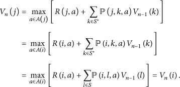
Table 1 shows the percentage reduction obtained for a network with three biosensors. ${ℰ}_{\mathrm{0}}$ is varied while fixing τ and L at 7 and 2, respectively. This considerable reduction is achieved just by aggregating the final valid and terminating states. Clearly, most of the system states fall into these two classes of system states. This can be attributed to the fact that the state space of the MDP model has a tree-like structure in which the number of leaf nodes representing terminating states is substantially large. The next substantially large number is the number of final valid states.

Table 1

Reduction in the number of system states when terminating states and final valid states are aggregated. The number of biosensors is 3. τ and L are 7 and 2, respectively.

${ℰ}_{\mathrm{0}}$	Total no. of states	Reduced no. of states	Percentage of reduction
5	884736	184319	79.17
6	1404928	341802	75.67
7	2097152	569849	72.83
8	2985984	881510	70.48
9	4096000	1289835	68.51
10	5451776	1807874	66.84

6. Numerical and Simulation Results

The numerical and simulation results are obtained by using the following example. Consider again the biosensor network shown in Figure 2. The biosensors are indexed from one to three. The neighbors of each biosensor are as follows:

• (i)

${\mathrm{\Omega }}_{\mathrm{1}}=\{2\}$ ,

(ii)

${\mathrm{\Omega }}_{\mathrm{2}}=\{1,3\}$ ,

(iii)

${\mathrm{\Omega }}_{\mathrm{3}}=\{2\}$ .

Also, the ℱ function in (3) is defined for each biosensor i as

$$\begin{array}{cc}& ℱ\left(T_t\left(i\right),W_t\left(a\right)\right)=T_t\left(i\right)+W_t\left(a\right).\end{array}$$

(14)

The channel for each biosensor is modeled as a two-state Markov chain whose state boundary is randomly generated. A biosensor requires ${ϵ}_k$ units of energy to successfully transmit its measurement when its channel is in state $k\in \{\mathrm{1,2}\}$ . It is assumed that ${ϵ}_k=k$ . The transition probability matrix is

$$\begin{array}{cc}& \left[\begin{array}{cc}\mathrm{0.2}& \mathrm{0.8}\\ \mathrm{0.6}& \mathrm{0.4}\end{array}\right].\end{array}$$

(15)

The MDP model of the biosensor network is solved using the RVI algorithm. The initial state of the network is assumed to be $\{(0,{ℰ}_0,1),(0,{ℰ}_0,1),(0,{ℰ}_0,1)\}$ . The expected network lifetime is the value calculated by the RVI algorithm for the initial state.

Figure 4 shows the expected network lifetime for different levels of initial energy ( ${ℰ}_{\mathrm{0}}$ ) and maximum allowed temperature increase (τ). For example, for $\tau =3$ (i.e., a maximum temperature of three units is allowed), the maximum expected network lifetime is 2.875. This can be achieved with an initial energy of 4 units. As the curve for $\tau =3$ shows, increasing the initial energy will not increase the expected lifetime due to the limit on the maximum allowed temperature increase.

Figure 4

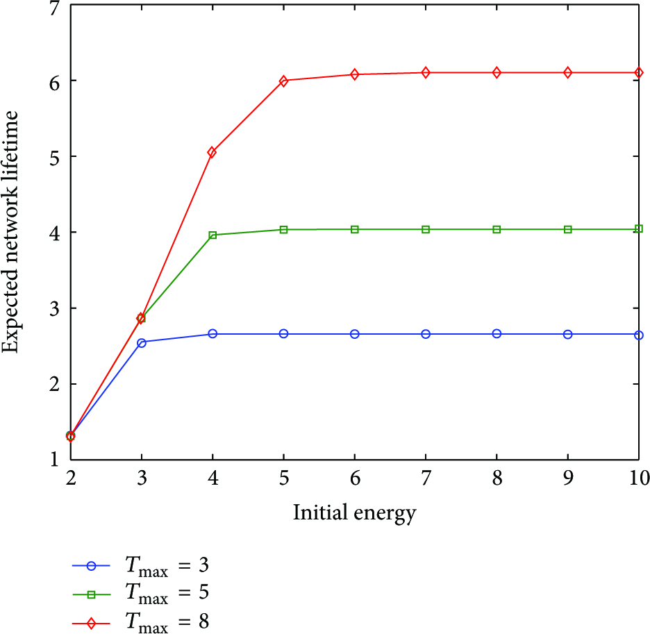
Expected network lifetime versus initial energy for different values of τ.

The initial energy of a biosensor might also become a limiting factor. For example, for $\tau =\mathrm{8}$ , ${ℰ}_{\mathrm{0}}$ limits the maximum expected lifetime over the range of initial energies from 2 to 6. After that, τ becomes the limiting factor. In this example, the maximum expected network lifetime which can be achieved with $\tau =\mathrm{8}$ is 7.265 with an initial energy of 7 units.

Another interesting issue is the amount of energy which remains in biosensors after the system is halted due to a high temperature increase. For example, from Figure 4, it can be seen that for ${ℰ}_{\mathrm{0}}=\mathrm{4}$ , increasing τ leads to a noticeable increase in the expected lifetime of the network. This indicates that the amount of initial energy must be determined carefully. This is because an excessive amount of remaining energy means that the patient has been exposed to an unnecessary temperature increase when the biosensors implanted in his body were charged. Thus, the measurement process has been started on already heated organs.

Figure 5 shows the actions the optimal policy makes when the remaining energy at each biosensor is fixed at three and the transmission energies of biosensors 1 and 2 are both two and that of biosensor 3 is one. ${ℰ}_{\mathrm{0}}$ and τ are both 5. After analyzing the data, it is found that biosensor 3 is selected for transmission in $\mathrm{64}\%$ of the system states since it results in the minimum temperature increase. This is obvious since only one unit of energy is required for a successful transmission and the size of its neighborhood is one. Biosensor 2 is never selected. Biosensor 1, however, is selected when the temperature at biosensor 3 or its neighbor (biosensor 2) is 4. This is because if any one of them is selected, the system will enter a terminating state. So, biosensor 1 is selected to let biosensor 3 cool down and thus lengthen the network lifetime or to distribute heat evenly if the network is going to enter a terminating state.

Figure 5

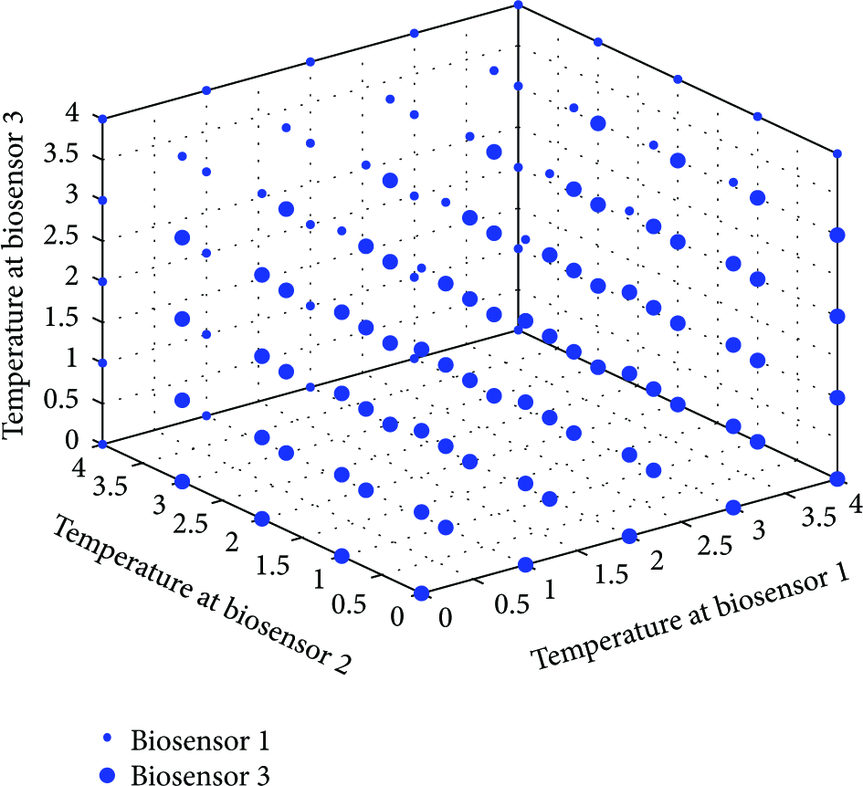
Optimal actions when $E(\mathrm{1})=E(\mathrm{2})=E(\mathrm{3})=\mathrm{3}$ , $W(\mathrm{1})=W(\mathrm{2})=\mathrm{2}$ and $W(\mathrm{3})=\mathrm{1}$ , $T=\mathrm{5}$ and ${ℰ}_{\mathrm{0}}=\mathrm{5}$ .

Next, the biosensor network is simulated to compare the performance of the optimal policy with that of the TIP-based and most residual energy policies. Also, the impact of varying the initial energy and maximum safe temperature level is evaluated. The simulator is written in Matlab [28] and each data point is the average of 1000 simulation runs. The TIP-based policy (or the optimal rotation sequence) is computed as described in [18]. The optimal sequence is $(\mathrm{3,1},2)$ . The peak potential is 0.148 and is experienced by biosensor 2. On the other hand, the most residual energy policy selects the biosensor whose transmission will result in the smallest reduction in energy.

First, the impact of varying the initial energy on the network lifetime is studied using simulation. Figure 6 shows the simulated lifetime of the biosensor network when the initial energy is varied from 2 to 10. Essentially, the network lifetime increases as the initial energy increases. However, after a threshold (around 4), the lifetime curve starts to level off for all policies. This is because the limit on the maximum allowed temperature increase is reached. Therefore, unless τ is increased, the average network lifetime will not increase with the increase of the initial energy.

Figure 6

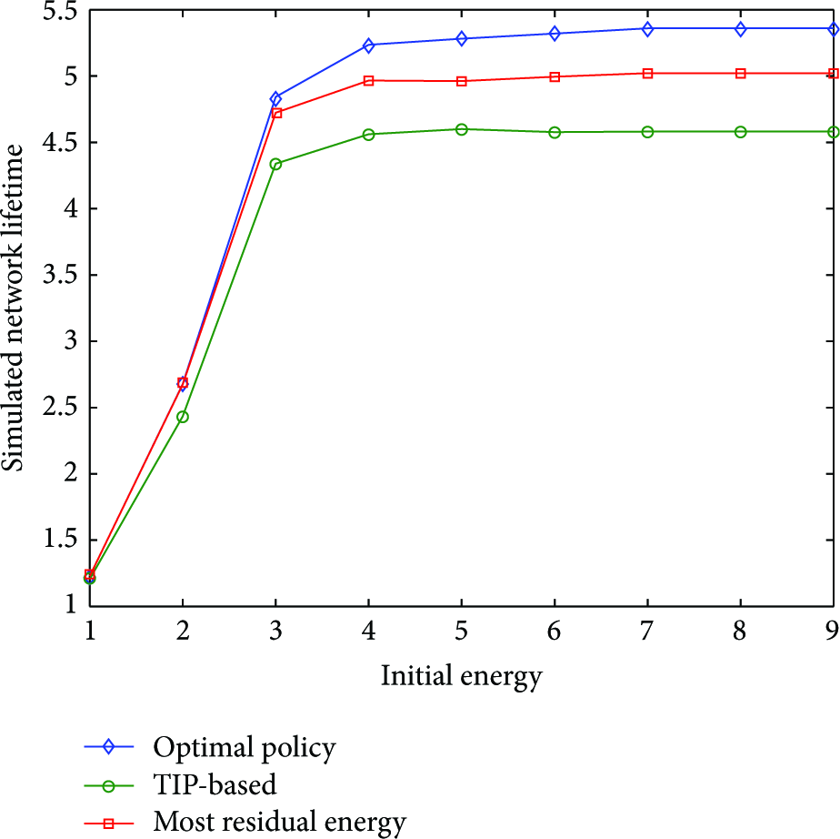
Simulated network lifetime versus initial energy for the different policies.

Figure 6 also shows that the optimal policy outperforms the other two policies. The TIP-based policy performs the worst. The main reason for its poor performance is that the TIP-based policy does not account for the effects of the wireless channel. On the other hand, the policy based on the most residual energy performs better than the TIP-based policy. This is because it always chooses the sensor which consumes the least amount of energy for transmission. Hence, the gap between its curve and that of the optimal policy is smaller. Nevertheless, its performance cannot reach the performance of the optimal policy since temperature is not considered explicitly.

Figure 7 shows the impact on the network lifetime when fixing the initial energy and varying the upper limit on the safe temperature level. As expected, the network lifetime increases as τ increases. However, this increase eventually levels off due to the lack of energy. Clearly, the optimal policy gives the best network lifetime. The policy based on the most residual energy gives the next best network lifetime. The worst network lifetime is achieved by the TIP-based policy.

Figure 7

Simulated network lifetime versus maximum safe temperature level for the different policies.

The performance of the three policies in terms of temperature increase is compared. The initial energy is fixed at ${ℰ}_{\mathrm{0}}=\mathrm{7}$ . The temperature at biosensor 2 is chosen as a metric. This is because biosensor 2 belongs to the neighborhoods of both biosensors 1 and 2. Thus, it might be heated continuously.

Figure 8 shows the temperature at biosensor 2 over four time slots. As expected, the TIP-based policy gives the maximum temperature increase. A closer examination of the simulation data reveals that biosensor 2 has indeed been continuously heated. This in turns leads to a larger temperature increase and thus shorter lifetime since the maximum allowed temperature is approached very fast.

Figure 8

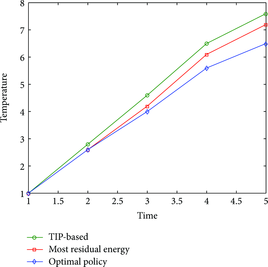
Temperature at biosensor 2 for the different policies.

Both the most residual energy and optimal policies give a significant improvement over the TIP-based policy. The performance of the two policies is slightly the same over the first two time slots. Then, the optimal policy shows a lower temperature increase over the remaining time slots.

The previous observation is very interesting since the goal of the TIP-based policy is to give a minimal temperature increase rotation sequence. However, since the wireless channel and its dynamics are not taken into account, the precomputed rotation sequence will most probably lead to a larger temperature increase when implemented in practice.

7. Conclusions and Directions for Further Research

The future of BWSNs is bright. However, much remains to be done to define the full potential of this technology. In this paper, we have taken one step further in understanding the thermal management problem in BWSNs. The problem is modeled as an MDP to obtain an optimal operating policy for the network. Further, the aggregation of final valid and terminating system states is proposed as a way for minimizing the number of states in the proposed MDP model. The equivalence of the reduced MDP model is established. Also, numerical results show a substantial reduction in model size which is obtained by aggregating just two types of system states. The optimal policy produced by the MDP model outperforms the policies based on the most residual energy and temperature increase potential. This is because the optimal policy gives the best balance between transmission energy consumption and the resulting temperature increase.

The following directions for further research are suggested. First, the notion of state equivalence used in this work is too strict and too sensitive. It is too strict because it requires that its conditions be met exactly. And, it is too sensitive because any perturbation of the transition probabilities can make two equivalent states no longer equivalent. More flexible metrics for state equivalence are needed. The works in [16, 17] can be used as a starting point. Second, in some applications like ours, the state transition probability matrix is built programmatically. This means a runtime which largely grows with the number of system states and thus state aggregation might not always be helpful. Hence, approximate techniques based on reinforcement learning are recommended (see [8–12]). Third, the possibility of obtaining effective policies based on simple heuristic techniques should be investigated. Heuristic techniques are typically characterized by their low runtime and storage requirements.