On the Joint Time Synchronization and Source Localization Using TOA Measurements

Abstract

This paper considers the problem of estimating the clock bias and the position of an unknown source using time of arrival (TOA) measurements obtained at a sensor array to achieve time synchronization and source localization. The study starts with deriving the localization mean square error (MSE) for the case where we pretend that the source clock bias is absent and apply TOA positioning to find the source position. An upper bound on the clock bias, over which we shall obtain a higher localization MSE than that from jointly identifying the clock bias with the source position, is established. Motivated by the MSE analysis, this paper proceeds to develop a new efficient solution for joint synchronization and source localization. The new method is in closed-form, computationally attractive, and more importantly; it is shown analytically to attain the CRLB accuracy under small Gaussian TOA measurement noise. Computer simulations are conducted to corroborate the theoretical development and illustrate the good performance of the proposed algorithm.

1. Introduction

Recently, source localization using wireless sensor networks (WSNs) has attracted great research efforts [1–4]. To determine the source position, positioning parameters such as time of arrival (TOA), time difference of arrival (TDOA), received signal strength (RSS), and angle of arrival (AOA) are commonly used. In this paper, we shall consider determining the source position using TOAs of the source signal received at a wireless sensor network, which is essential for emerging applications including logistics, search and rescue, medical service, smart homes, environmental monitoring, and surveillance [5]. For this problem, a large number of algorithms such as those in [6–14] have been developed in literatures. Nevertheless, almost all of them assumed that the source and the sensors are synchronized ahead of the localization process. In other words, the clock biases of the source and the sensors are known a priori so that the obtained TOA measurements can be transformed into range measurement for source localization via TOA positioning.

In practice, the source clock bias may not be readily available and the TOA measurements are therefore subject to unknown source clock bias. In this case, we may simply ignore the source clock bias and still locate the source through TOA positioning. It can be expected by intuition that the obtained source localization accuracy would be worse than the case where the source clock bias is known a priori. However, the amount of performance degradation would be small if the source clock bias is negligible compared to the source-sensor distances. On the other hand, another way to handle the presence of the unknown source clock bias is to estimate it jointly with the source position. This would also yield a source localization accuracy poorer than that when the source clock bias is known a priori, due to the increase in the number of unknowns to be identified. Clearly, a theoretical analysis is needed here to compare the performance of the above two methods in terms of their localization accuracy. The obtained results would reveal the sensitivity of TOA positioning to the presence of the unknown source clock bias in the TOA measurement. More importantly, they would establish the conditions under which joint time synchronization and source localization should be preferred in order to achieve better source localization accuracy. To the best of our knowledge, this has not been addressed in existing literatures.

When the source clock bias cannot be ignored and/or it is also of interest besides the source position, an algorithm that can estimate both the source position and clock bias from the TOA measurements is definitely needed. For example, this could occur when a sensor is newly added to the WSN and it needs to be located and synchronized. Conventionally, synchronization and source localization are treated separately. In particular, synchronization is usually achieved first via applying one of the available protocol-domain techniques, such as [15–17], and the localization task can then be accomplished by executing various algorithms, such as those developed in [7–9, 12–14]. A more recent trend is to perform joint synchronization and source localization owing to their close relationship [18–22]. For this problem, given the statistical model of the TOA measurement noise, the maximum likelihood estimator (MLE) can be developed. However, since the cost function is nonconvex, MLE often resorts to the iterative search with a good initial guess for finding a globally optimal solution. This approach possesses the local convergence and even divergence problems. Another disadvantage is the high computational complexity due to possibly large number of iterations. Therefore, a closed-form solution is highly desirable. Bancroft's closed-form solution [23] is the first linearization-based algorithm for 1D timing (i.e., clock bias estimation) and 3D positioning. Zhu and Ding extended Bancroft's method in [21] to the case where the number of TOA measurements is more than the dimension of the unknowns (i.e., the source position plus the clock bias). However, this approach is in general not efficient. In other words, it can attain the Cramér-Rao Lower Bound (CRLB), the best accuracy for an unbiased estimator, in certain scenarios only.

The contribution of this paper is twofold. Firstly, we conduct a mean square error (MSE) analysis to derive the source localization MSE when the source clock bias in the TOA measurements is neglected and TOA positioning is performed to locate the source. For this purpose, a first-order analysis on a pseudo-MLE source location estimator is utilized, which indicates that the obtained results are valid for small TOA noise and source clock bias. The obtained source localization MSE would be partially dependent on the value of the source clock bias and as a result, it reflects the sensitivity of the TOA positioning accuracy to the presence of source clock bias. Moreover, an upper bound on the absolute value of the source clock bias is derived, over which joint synchronization and source localization would provide better localization accuracy in terms of smaller localization MSE than TOA positioning after ignoring the source clock bias. Secondly, this paper proposes a new efficient solution in closed-form for joint synchronization and localization. The newly developed method consists of two processing steps, where the first step locates the source and the second step estimates the clock bias. Compared with the iterative MLE method, the proposed solution is computationally more attractive, since it does not possess local convergence or divergence problem. Moreover, in contrast to the closed-form Bancroft's method [23] and its generalized version [21], the new approach is shown analytically to be able to attain the CRLB accuracy for both source location and source clock under small TOA noise. We support our theoretical developments using extensive computer simulations.

It is worthwhile to point out that the theoretical approach adopted in this paper to perform the MSE analysis and develop the proposed algorithm can be applied in a straightforward manner to the case when the TOAs are deduced from twoway/round-trip time of flight (TOF) measurements. TOF is usually considered as an inexpensive but effective alternative to obtain TOAs without using the cumbersome and costly source-sensor synchronization [24–26]. In this case, however, the turn-around time at the source needs to be either estimated [26] or small enough to be negligible [27, 28] so that TOA positioning can be utilized. With the above observation in mind, it is not difficult to show that the turn-around time in the TOF-deduced TOA measurements can be considered mathematically as an equivalent source clock bias. As a result, the MSE analysis and the proposed algorithm presented in this paper can be applied without much modifications to investigate the effect of ignoring the turn-around time and perform joint estimation of the turn-around time and the source position.

The structure of this paper is as follows. Section 2 formulates the joint time synchronization and source localization problem under Gaussian TOA noise model. Besides, the corresponding CRLB is established and analyzed in detail to motivate the MSE analysis and the new estimation algorithm development. Section 3 derives and verifies by computer simulations the localization MSE when the source clock bias in the received TOAs is ignored and the source position is found via TOA positioning. Section 4 presents the proposed closed-form solution for joint synchronization and source localization. Theoretical performance analysis that establishes the efficiency of the new method under small TOA measurement error is also conducted. Section 5 gives the simulation results to illustrate the good performance of the newly developed algorithm, and Section 6 concludes the paper and discusses the future work.

2. Problem Formulation and CRLB

In this section, we shall first formulate the joint time synchronization and source localization problem in consideration. The CRLB for the unknowns is then derived and analysed to motivate the MSE analysis and the algorithm development presented in the following two sections.

2.1. Signal Model

We shall consider jointly synchronizing and locating a single source in a 2D plane. The extensions of the theoretical developments in this paper to the more general case of synchronizing and localizing a source in the 3D space are straightforward.

The source is located at an unknown position $\mathbf{p}=[{\mathrm{p}}_{\mathrm{x}},{\mathrm{p}}_{\mathrm{y}}{]}^{\mathrm{T}}$ . It has an unknown clock bias of $\tilde{\tau }$ seconds with respect to the reference time (i.e., the true time). Mathematically, the local time at the source would be $\mathrm{t}-\tilde{\tau }$ if the reference time is t. The value of $\tilde{\tau }$ can be negative or positive. Besides, $\tilde{\tau }$ is unknown but deterministic.

A sensor array composed of M sensors at accurately known positions ${\mathbf{p}}_{\mathrm{m}}=[{\mathrm{p}}_{\mathrm{m},\mathrm{x}},{\mathrm{p}}_{\mathrm{m},\mathrm{y}}{]}^{\mathrm{T}}$ , $\mathrm{m}=\mathrm{1,2},\dots ,\mathrm{M}$ , is used to identify p and $\tilde{\tau }$ by measuring the TOAs of the source signal. Without loss of generality, we assume that the source starts emitting signals at its local time 0, which corresponds to the reference time $\tilde{\tau }$ . The source signal reaches sensor m at the reference time $\tilde{\tau }+{\mathrm{d}}_{\mathrm{m}}/\mathrm{c}$ , where ${\mathrm{d}}_{\mathrm{m}}=\parallel \mathbf{p}-{\mathbf{p}}_{\mathrm{m}}\parallel$ is the true distance between the source and sensor m, $\parallel \star \parallel$ denotes the 2-norm and c is the signal propagation speed. Let ${\tilde{\tau }}_{\mathrm{m}}$ be the known clock bias of sensor m with respect to the reference time. The TOA measurement obtained at sensor m would be [21], after taking into account the measurement error ${\tilde{\mathrm{n}}}_{\mathrm{m}}$ ,

$$\begin{array}{cc}& {\tilde{\mathrm{T}}}_{\mathrm{m}}=\tilde{\tau }-{\tilde{\tau }}_{\mathrm{m}}+\frac{{\mathrm{d}}_{\mathrm{m}}}{\mathrm{c}}+{\tilde{\mathrm{n}}}_{\mathrm{m}}.\end{array}$$

(1)

Multiplying both sides of the above equation with the signal propagation speed c yields the TOA equation

$$\begin{array}{cc}& {\mathrm{T}}_{\mathrm{m}}=\tau -{\tau }_{\mathrm{m}}+{\mathrm{d}}_{\mathrm{m}}+{\mathrm{n}}_{\mathrm{m}},\end{array}$$

(2)

where ${\mathrm{T}}_{\mathrm{m}}=\mathrm{c}{\tilde{\mathrm{T}}}_{\mathrm{m}}$ , $\tau =\mathrm{c}\tilde{\tau }$ , ${\tau }_{\mathrm{m}}=\mathrm{c}{\tilde{\tau }}_{\mathrm{m}}$ , and ${\mathrm{n}}_{\mathrm{m}}=\mathrm{c}{\tilde{\mathrm{n}}}_{\mathrm{m}}$ . Note that the scaled clock biases in (2), namely τ and ${\tau }_{\mathrm{m}}$ , now have the units of meters. Noting that estimating the original source clock bias $\tilde{\tau }$ is equivalent to identifying its scaled version τ, we shall focus on determining τ in the rest of this paper to simplify the presentation.

Following the noise model in [21], we assume that the TOA measurement errors ${\mathrm{n}}_{\mathrm{m}}$ in (2) are independently and identically distributed (i.i.d.) Gaussian random variables with zero mean and variance ${\sigma }_{\mathrm{n}}^{\mathrm{2}}$ . This model has been commonly adopted in literatures such as [10–14] for developing TOA-based localization algorithms and/or studying their performance via computer simulations. Nevertheless, it is a simplification of the real scenario where besides zero-mean Gaussian random errors due to the additive Gaussian noise at every sensor [10], the TOA measurements are also subject to errors owing to the multipath and nonline-of-sight (NLOS) propagation of the source signal as shown in recent experimental studies [29–31]. The fundamental limits of localization accuracy under these realistic factors was established in [32]. Extending our work to more realistic TOA noise models is beyond the scope of this paper, but it is under investigation.

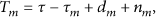
By introducing the $\mathrm{M}\times \mathrm{1}$ vectors,

$$\begin{array}{cc}& \mathbf{T}=\left[\begin{array}{c}⋮\\ {\mathrm{T}}_{\mathrm{m}}+{\tau }_{\mathrm{m}}\\ ⋮\\ \end{array}\right],\hspace{1em}\hspace{1em}\mathbf{d}=\left[\begin{array}{c}⋮\\ {\mathrm{d}}_{\mathrm{m}}\\ ⋮\\ \end{array}\right],\hspace{1em}\hspace{1em}\mathbf{n}=\left[\begin{array}{c}⋮\\ {\mathrm{n}}_{\mathrm{m}}\\ ⋮\\ \end{array}\right],\\ {\mathbf{1}}_{\mathrm{M}}=\left[\begin{array}{c}⋮\\ \mathrm{1}\\ ⋮\\ \end{array}\right]\end{array}$$

(3)

we can express the measured TOA in (2) using the following signal model in matrix form:

$$\begin{array}{cc}& \mathbf{T}=\tau {\mathbf{1}}_{\mathrm{M}}+\mathbf{d}+\mathbf{n}.\end{array}$$

(4)

The problem of interest is to estimate the source position vector p and the source clock bias τ given T and ${\mathbf{p}}_{\mathrm{m}}$ .

2.2. CRLB Analysis

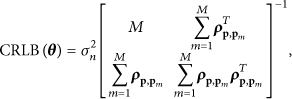
The CRLB for the composite unknown vector $\mathbf{\theta }=[\tau ,{\mathbf{p}}^{\mathrm{T}}{]}^{\mathrm{T}}$ under the joint time synchronization and localization scenario presented in the previous subsection is [21]

$$\begin{array}{cc}& \text{CRLB}\left(\mathbf{\theta }\right)={\sigma }_{\mathrm{n}}^{\mathrm{2}}{\left[\begin{array}{cc}\mathrm{M}& \sum _{\mathrm{m}=\mathrm{1}}^{\mathrm{M}}{\mathit{\rho }}_{\mathbf{p},{\mathbf{p}}_{\mathrm{m}}}^{\mathrm{T}}\\ \sum _{\mathrm{m}=\mathrm{1}}^{\mathrm{M}}{\mathit{\rho }}_{\mathbf{p},{\mathbf{p}}_{\mathrm{m}}}& \sum _{\mathrm{m}=\mathrm{1}}^{\mathrm{M}}{\mathit{\rho }}_{\mathbf{p},{\mathbf{p}}_{\mathrm{m}}}{\mathit{\rho }}_{\mathbf{p},{\mathbf{p}}_{\mathrm{m}}}^{\mathrm{T}}\end{array}\right]}^{-\mathrm{1}},\end{array}$$

(5)

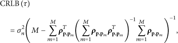
where ${\mathit{\rho }}_{\mathbf{p},{\mathbf{p}}_{\mathrm{m}}}=(\mathbf{p}-{\mathbf{p}}_{\mathrm{m}})/\parallel \mathbf{p}-{\mathbf{p}}_{\mathrm{m}}\parallel$ is a unit vector from ${\mathbf{p}}_{\mathrm{m}}$ to p. The CRLB of the source clock bias τ, denoted by CRLB $(\tau )$ , is given by the upper left component of CRLB $(\mathbf{\theta })$ while the lower right $\mathrm{2}\times \mathrm{2}$ block of CRLB $(\mathbf{\theta })$ is the CRLB of the source position p, denoted by CRLB $(\mathbf{p})$ . Applying the partitioned matrix inversion formula [33], we have

$$\begin{array}{ll}& \text{CRLB}\left(\tau \right)\\ \hspace{1em}={\sigma }_{\mathrm{n}}^{\mathrm{2}}{\left(\mathrm{M}-\sum _{\mathrm{m}=\mathrm{1}}^{\mathrm{M}}‍{\mathit{\rho }}_{\mathbf{p},{\mathbf{p}}_{\mathrm{m}}}^{\mathrm{T}}{\left(\sum _{\mathrm{m}=\mathrm{1}}^{\mathrm{M}}‍{\mathit{\rho }}_{\mathbf{p},{\mathbf{p}}_{\mathrm{m}}}{\mathit{\rho }}_{\mathbf{p},{\mathbf{p}}_{\mathrm{m}}}^{\mathrm{T}}\right)}^{-\mathrm{1}}\sum _{\mathrm{m}=\mathrm{1}}^{\mathrm{M}}‍{\mathit{\rho }}_{\mathbf{p},{\mathbf{p}}_{\mathrm{m}}}\right)}^{-\mathrm{1}},\end{array}$$

(6a)

$$\begin{array}{ll}& \text{CRLB}\left(\mathbf{p}\right)\\ \hspace{1em}={\sigma }_{\mathrm{n}}^{\mathrm{2}}{\left(\sum _{\mathrm{m}=\mathrm{1}}^{\mathrm{M}}‍{\mathit{\rho }}_{\mathbf{p},{\mathbf{p}}_{\mathrm{m}}}{\mathit{\rho }}_{\mathbf{p},{\mathbf{p}}_{\mathrm{m}}}^{\mathrm{T}}-\frac{\mathrm{1}}{\mathrm{M}}\sum _{\mathrm{m}=\mathrm{1}}^{\mathrm{M}}‍{\mathit{\rho }}_{\mathbf{p},{\mathbf{p}}_{\mathrm{m}}}\sum _{\mathrm{m}=\mathrm{1}}^{\mathrm{M}}‍{\mathit{\rho }}_{\mathbf{p},{\mathbf{p}}_{\mathrm{m}}}^{\mathrm{T}}\right)}^{-\mathrm{1}}.\end{array}$$

(6b)

We proceed to evaluate (6b) more carefully to gain more insights. Collecting ${\mathit{\rho }}_{\mathbf{p},{\mathbf{p}}_{\mathrm{m}}}$ , $\mathrm{m}=\mathrm{1,2},\dots ,\mathrm{M}$ , yields the $\mathrm{M}\times \mathrm{2}$ partial derivative matrix H given as

$$\begin{array}{cc}& \mathbf{H}=\left[\begin{array}{c}⋮\\ {\mathit{\rho }}_{\mathbf{p},{\mathbf{p}}_{\mathrm{m}}}^{\mathrm{T}}\\ ⋮\end{array}\right].\end{array}$$

(7)

CRLB $(\mathbf{p})$ can then be expressed as

$$\begin{array}{lll}\mathbf{R}\hfill & =\hfill & \left[\begin{array}{c}-{\mathbf{1}}_{\mathrm{M}-1}^{\mathrm{T}}\\ {\mathbf{I}}_{\mathrm{M}-1}\end{array}\right]\left({\mathbf{I}}_{\mathrm{M}-1}-\frac{1}{\mathrm{M}}{\mathbf{1}}_{\mathrm{M}-1}{\mathbf{1}}_{\mathrm{M}-1}^{\mathrm{T}}\right)\hfill \\ \hfill & \hfill & \times [-{\mathbf{1}}_{\mathrm{M}-1}\hspace{0.17em}\hspace{0.17em}{\mathbf{I}}_{\mathrm{M}-1}],\hfill \end{array}$$

(8)

where $\mathbf{R}={\mathbf{I}}_{\mathrm{M}}-(\mathrm{1}/\mathrm{M}){\mathbf{1}}_{\mathrm{M}}{\mathbf{1}}_{\mathrm{M}}^{\mathrm{T}}$ , ${\mathbf{I}}_{\mathrm{M}}$ is an $\mathrm{M}\times \mathrm{M}$ identity matrix and ${\mathbf{1}}_{\mathrm{M}}$ is an $\mathrm{M}\times \mathrm{1}$ column vector whose elements are all equal to one as defined in (4). The matrix R can be rewritten as the following matrix product:

$$\begin{array}{ll}& \mathbf{R}=\left[\begin{array}{l}-{\mathbf{1}}_{\mathrm{M}-\mathrm{1}}^{\mathrm{T}}\\ {\mathbf{I}}_{\mathrm{M}-\mathrm{1}}\end{array}\right]\left({\mathbf{I}}_{\mathrm{M}-\mathrm{1}}-\frac{\mathrm{1}}{\mathrm{M}}{\mathbf{1}}_{\mathrm{M}-\mathrm{1}}{\mathbf{1}}_{\mathrm{M}-\mathrm{1}}^{\mathrm{T}}\right)\\ \times \left[\begin{array}{ll}-{\mathbf{1}}_{\mathrm{M}-\mathrm{1}}& {\mathbf{I}}_{\mathrm{M}-\mathrm{1}}\end{array}\right],\end{array}$$

(9)

where ${\mathbf{I}}_{\mathrm{M}-\mathrm{1}}$ is an $(\mathrm{M}-\mathrm{1})\times (\mathrm{M}-\mathrm{1})$ identity matrix and ${\mathbf{1}}_{\mathrm{M}-\mathrm{1}}$ is an $(\mathrm{M}-\mathrm{1})\times \mathrm{1}$ column vector whose elements are all equal to one. Applying the matrix inversion lemma [33] to the matrix in the middle of the right hand sides of (9) yields

$$\begin{array}{cc}& \left({\mathbf{I}}_{\mathrm{M}-\mathrm{1}}-\frac{\mathrm{1}}{\mathrm{M}}{\mathbf{1}}_{\mathrm{M}-\mathrm{1}}{\mathbf{1}}_{\mathrm{M}-\mathrm{1}}^{\mathrm{T}}\right)={\left({\mathbf{I}}_{\mathrm{M}-\mathrm{1}}+{\mathbf{1}}_{\mathrm{M}-\mathrm{1}}{\mathbf{1}}_{\mathrm{M}-\mathrm{1}}^{\mathrm{T}}\right)}^{-\mathrm{1}}={\mathbf{Q}}_{\alpha }^{-\mathrm{1}}.\end{array}$$

(10)

Clearly, ${\mathbf{Q}}_{\alpha }$ is an $(\mathrm{M}-\mathrm{1})\times (\mathrm{M}-\mathrm{1})$ matrix with all its diagonal elements equal to 2 and others equal to 1. Substituting (10) back into (9) and putting the result into (8), we have

$$\begin{array}{cc}& \text{CRLB}\left(\mathbf{p}\right)={\sigma }_{\mathrm{n}}^{\mathrm{2}}{\left({\tilde{\mathbf{H}}}^{\mathrm{T}}{\mathbf{Q}}_{\alpha }^{-\mathrm{1}}\tilde{\mathbf{H}}\right)}^{-\mathrm{1}},\end{array}$$

(11)

where $\tilde{\mathbf{H}}=[-{\mathbf{1}}_{\mathrm{M}-\mathrm{1}}\mathrm{\hspace{0.17em}\hspace{0.17em}}\mathrm{\hspace{0.17em}\hspace{0.17em}}{\mathbf{I}}_{\mathrm{M}-\mathrm{1}}]\mathbf{H}$ is an $(\mathrm{M}-\mathrm{1})\times \mathrm{2}$ matrix whose $(\mathrm{m}-\mathrm{1})$ th row, $\mathrm{m}=\mathrm{2,3},\dots ,\mathrm{M}$ , is equal to

$$\begin{array}{cc}& \tilde{\mathbf{H}}(\mathrm{m}-\mathrm{1},:)={\mathit{\rho }}_{\mathbf{p},{\mathbf{p}}_{\mathrm{m}}}^{\mathrm{T}}-{\mathit{\rho }}_{\mathbf{p},{\mathbf{p}}_{\mathrm{1}}}^{\mathrm{T}}.\end{array}$$

(12)

Comparing (11) with (33) from [34], we notice that within the considered time synchronization and source localization framework, the CRLB of the source position is equal to that of locating the source from $\mathrm{M}-\mathrm{1}$ time difference of arrival (TDOA) measurements ${\mathrm{r}}_{\mathrm{m}\mathrm{1}}=({\mathrm{T}}_{\mathrm{m}}+{\tau }_{\mathrm{m}})-({\mathrm{T}}_{\mathrm{1}}+{\tau }_{\mathrm{1}})$ , where $\mathrm{m}=\mathrm{2,3},\dots ,\mathrm{M}$ . In other words, the TDOA measurements ${\mathrm{r}}_{\mathrm{m}\mathrm{1}}$ are indeed generated by subtracting the TOA obtained at sensor $\mathrm{1}$ from the remaining TOAs. From the definition of the TOA measurements ${\mathrm{T}}_{\mathrm{m}}$ given in (2), all the TOAs are linearly related to the unknown source clock bias τ and hence, the subtraction operation eliminates the presence of τ in the obtained TDOAs ${\mathrm{r}}_{\mathrm{m}\mathrm{1}}$ . This enables TDOA positioning of the source and also forms the basis of the joint synchronization and localization algorithm proposed in Section 4 of this paper.

It is worthwhile to point out that we choose to produce the TDOAs through subtracting the TOA measured at sensor 1 from the rest $\mathrm{M}-\mathrm{1}$ TOAs for two reasons. First, this facilitates the comparison of the CRLB result derived in (11) with (33) from [34], where the TDOA measurements were also obtained with respect to sensor 1. Second, subtracting the TOA at any sensor other than sensor 1 from the remaining $\mathrm{M}-\mathrm{1}$ TOAs would yield a different set of TDOA measurements but with the same quality as ${\mathrm{r}}_{\mathrm{m}\mathrm{1}}$ in terms of the source localization CRLB. This can be verified by applying the fact from Section 2 that the TOA measurement noises ${\mathrm{n}}_{\mathrm{m}}$ are i.i.d. and they have the same variance. Nevertheless, the above observation would become invalid if ${\mathrm{n}}_{\mathrm{m}}$ are no longer i.i.d. Investigating the approach that takes into account the statistical information on ${\mathrm{n}}_{\mathrm{m}}$ to produce the optimal TDOA measurement set is an important topic subject to future researches.

When the clock bias of the source, τ, is available a priori, but the source position p remains unknown, the joint synchronization and localization task reduces to the classic problem of TOA positioning using the measurements in (2). The best possible localization accuracy for this case becomes [21]

$$\begin{array}{cc}& \text{CRLB}{\left(\mathbf{p}\right)}_{\mathrm{o}}={\sigma }_{\mathrm{n}}^{\mathrm{2}}{\left(\sum _{\mathrm{m}=\mathrm{1}}^{\mathrm{M}}‍{\mathit{\rho }}_{\mathbf{p},{\mathbf{p}}_{\mathrm{m}}}{\mathit{\rho }}_{\mathbf{p},{\mathbf{p}}_{\mathrm{m}}}^{\mathrm{T}}\right)}^{-\mathrm{1}}.\end{array}$$

(13)

$\text{CRLB}(\mathbf{p}{)}_{\mathrm{o}}$ and $\text{CRLB}(\mathbf{p})$ given in (6b) are the CRLBs of the source location estimation under two different scenarios, namely, when the source block bias τ is known and when τ is unknown. They are both $\mathrm{2}\times \mathrm{2}$ matrices and have the same units, which makes subtracting $\text{CRLB}(\mathbf{p}{)}_{\mathrm{o}}$ in (13) from CRLB $(\mathbf{p})$ in (6b) feasible. In fact, it can shown that CRLB $(\mathbf{p})$ - $\text{CRLB}(\mathbf{p}{)}_{\mathrm{o}}$ is a positive semidefinite matrix, which indicates that compared with TOA positioning, the problem of joint time synchronization and source localization considered in this paper has a worse localization accuracy in general. This is expected, because we need to estimate one more unknown, specifically the source clock bias τ, from the same set of TOA measurements.

On the other hand, carefully examining (2) reveals that if the clock bias τ is negligible compared to the source-sensor distance ${\mathrm{d}}_{\mathrm{m}}$ , $\mathrm{m}=\mathrm{1,2},\dots ,\mathrm{M}$ , or equivalently $\tau /{\mathrm{d}}_{\mathrm{m}}\approx \mathrm{0}$ , and the source position is of primary interest, we may simply ignore the presence of τ and apply TOA positioning technique to the TOA measurements ${\mathrm{T}}_{\mathrm{m}}$ in (2) for identifying p. In this way, the obtained location estimate will be biased, but it could have a smaller localization MSE than that of the location estimate from an efficient estimator for joint time synchronization and source localization. We shall theoretically illustrate the above observations in the following section.

3. Localization MSE Analysis

In this section, we shall derive the localization MSE when identifying the source position p from the TOA measurements ${\mathrm{T}}_{\mathrm{m}}$ in (2) via TOA positioning and pretending that the source clock bias τ is zero. The obtained results will be contrasted with the best achievable localization MSE under the framework of joint estimation of τ and p, which is equal to the trace of the CRLB $(\mathbf{p})$ given in (6b). The theoretical developments are based on an estimator that utilizes the Taylor-series linearization and estimates the source location from ${\mathrm{T}}_{\mathrm{m}}$ via the classic weighted least squares (WLS) technique. The reason behind the use of a WLS source location estimate is that it enables obtaining its localization MSE in closed form in terms of the TOA measurement noise power ${\sigma }_{\mathrm{n}}^{\mathrm{2}}$ and the source clock bias τ to gain more insights. The localization MSE result in this section is valid for the scenario where the TOA measurement noise and the source clock bias are both small, due to the use of first-order approximation in the considered location estimator. But it applies to any TOA positioning technique that achieves the CRLB accuracy (13) when the source clock bias is known a priori. We shall corroborate the analytical results using numerical examples in Section 3.1 where the maximum-likelihood (ML) estimator for TOA positioning that attains (13) asymptotically when the source clock bias is known is simulated.

The MSE analysis starts with approximating the TOA measurement in (2) via applying the Taylor-series expansion up to the linear term to the source-sensor distance ${\mathrm{d}}_{\mathrm{m}}=\parallel \mathbf{p}-{\mathbf{p}}_{\mathrm{m}}\parallel$ using an initial source position guess $\tilde{\mathbf{p}}$ . Mathematically, we have

$$\begin{array}{cc}& {\mathrm{T}}_{\mathrm{m}}\approx \tau -{\tau }_{\mathrm{m}}+\parallel \tilde{\mathbf{p}}-{\mathbf{p}}_{\mathrm{m}}\parallel +{\mathit{\rho }}_{\tilde{\mathbf{p}},{\mathbf{p}}_{\mathrm{m}}}^{\mathrm{T}}(\mathbf{p}-\tilde{\mathbf{p}}).\end{array}$$

(14)

It can be deduced from (14) that the identification of the source position p is equivalent to find $(\mathbf{p}-\tilde{\mathbf{p}})$ . For this purpose, we rearrange (14) and stack the result for $\mathrm{m}=\mathrm{1,2},\dots ,\mathrm{M}$ to arrive at

$$\begin{array}{cc}& \underset{\mathbf{h}}{\underbrace{\left[\begin{array}{c}⋮\\ {\mathrm{T}}_{\mathrm{m}}+{\tau }_{\mathrm{m}}-\parallel \tilde{\mathbf{p}}-\mathbf{p}\parallel \\ ⋮\end{array}\right]}}=\underset{\mathbf{G}}{\underbrace{\left[\begin{array}{c}⋮\\ {\mathit{\rho }}_{\tilde{\mathbf{p}},{\mathbf{p}}_{\mathrm{m}}}^{\mathrm{T}}\\ ⋮\end{array}\right]}}\left(\mathbf{p}-\tilde{\mathbf{p}}\right)+\tau {\mathbf{1}}_{\mathrm{M}}+\mathbf{n},\end{array}$$

(15)

where ${\mathbf{1}}_{\mathrm{M}}$ and n are defined in (4). Pretending that $\tau =\mathrm{0}$ and utilizing n being zero-mean Gaussian random vector, the maximum likelihood (ML) estimate for $(\mathbf{p}-\tilde{\mathbf{p}})$ can be derived using the WLS technique [35]. Adding the result to the initial solution guess for p yields the final source position estimate

$$\begin{array}{cc}& \widetilde{\stackrel{~}{\mathbf{p}}}=\tilde{\mathbf{p}}+{\left({\mathbf{G}}^{\mathrm{T}}\mathbf{G}\right)}^{-\mathrm{1}}{\mathbf{G}}^{\mathrm{T}}\mathbf{h}.\end{array}$$

(16)

Substituting (15) into the above equation and subtracting the true source position p from both sides give the estimation error, when the clock bias τ is ignored

$$\begin{array}{cc}& \widetilde{\stackrel{~}{\mathbf{p}}}-\mathbf{p}={\left({\mathbf{G}}^{\mathrm{T}}\mathbf{G}\right)}^{-\mathrm{1}}{\mathbf{G}}^{\mathrm{T}}(\tau {\mathbf{1}}_{\mathrm{M}}+\mathbf{n}).\end{array}$$

(17)

Assuming that the initial source position guess $\tilde{\mathbf{p}}$ is sufficiently close to the true value p, we can ignore the error in G and approximate it with H defined in (7) whose row vectors are ${\mathit{\rho }}_{\mathbf{p},{\mathbf{p}}_{\mathrm{m}}}^{\mathrm{T}}$ . Therefore, (17) becomes

$$\begin{array}{cc}& \widetilde{\stackrel{~}{\mathbf{p}}}-\mathbf{p}\approx {\left({\mathbf{H}}^{\mathrm{T}}\mathbf{H}\right)}^{-\mathrm{1}}{\mathbf{H}}^{\mathrm{T}}(\tau {\mathbf{1}}_{\mathrm{M}}+\mathbf{n}).\end{array}$$

(18)

It can been observed that $\widetilde{\stackrel{~}{\mathbf{p}}}$ is a biased estimate of p and the estimation bias is equal to $\tau {({\mathbf{H}}^{\mathrm{T}}\mathbf{H})}^{-\mathrm{1}}{\mathbf{H}}^{\mathrm{T}}{\mathbf{1}}_{\mathrm{M}}$ , which is proportional to the value of the source clock bias τ. Moreover, the localization MSE can be derived by multiplying both sides of (18) with the transpose of $\widetilde{\stackrel{~}{\mathbf{p}}}-\mathbf{p}$ and taking expectation as well as the matrix trace. We have

$$\begin{array}{ll}& \text{MSE}\left(\widetilde{\stackrel{~}{\mathbf{p}}}\right)=\mathrm{tr}({\sigma }_{\mathrm{n}}^{\mathrm{2}}{\left({\mathbf{H}}^{\mathrm{T}}\mathbf{H}\right)}^{-\mathrm{1}}\\ \hspace{1em}\hspace{0.5em}+{\tau }^{\mathrm{2}}{\left({\mathbf{H}}^{\mathrm{T}}\mathbf{H}\right)}^{-\mathrm{1}}{\mathbf{H}}^{\mathrm{T}}{\mathbf{1}}_{\mathrm{M}}{\mathbf{1}}_{\mathrm{M}}^{\mathrm{T}}\mathbf{H}{\left({\mathbf{H}}^{\mathrm{T}}\mathbf{H}\right)}^{-\mathrm{1}}),\end{array}$$

(19)

where $\mathrm{tr}()$ is the trace of a matrix.

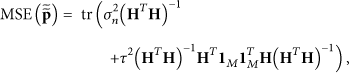
On the other hand, the localization MSE of an efficient estimator for jointly identifying p and τ can be derived by applying the matrix inversion lemma [33] to (8) and evaluating its trace. Subtracting the result from (19) yields

$$\begin{array}{ll}& \text{MSE}\left(\widetilde{\stackrel{~}{\mathbf{p}}}\right)-\mathrm{tr}\left(\text{CRLB}\left(\mathbf{p}\right)\right)\\ \hspace{1em}\hspace{1em}=\left({\tau }^{\mathrm{2}}-\frac{{\sigma }_{\mathrm{n}}^{\mathrm{2}}}{\mathrm{M}-{\mathbf{1}}_{\mathrm{M}}^{\mathrm{T}}\mathbf{H}{\left({\mathbf{H}}^{\mathrm{T}}\mathbf{H}\right)}^{-\mathrm{1}}{\mathbf{H}}^{\mathrm{T}}{\mathbf{1}}_{\mathrm{M}}}\right)\\ \hspace{1em}\hspace{1em}\hspace{1em}\times \mathrm{tr}\left({\left({\mathbf{H}}^{\mathrm{T}}\mathbf{H}\right)}^{-\mathrm{1}}{\mathbf{H}}^{\mathrm{T}}{\mathbf{1}}_{\mathrm{M}}{\mathbf{1}}_{\mathrm{M}}^{\mathrm{T}}\mathbf{H}{\left({\mathbf{H}}^{\mathrm{T}}\mathbf{H}\right)}^{-\mathrm{1}}\right).\end{array}$$

(20)

This indicates that ignoring the clock bias τ may still lead to a location estimate with a smaller localization MSE than that of jointly identifying it together with the source position p, if the following inequality holds:

$$\begin{array}{cc}& {\tau }^{\mathrm{2}}<\frac{{\sigma }_{\mathrm{n}}^{\mathrm{2}}}{\mathrm{M}-{\mathbf{1}}_{\mathrm{M}}^{\mathrm{T}}\mathbf{H}{\left({\mathbf{H}}^{\mathrm{T}}\mathbf{H}\right)}^{-\mathrm{1}}{\mathbf{H}}^{\mathrm{T}}{\mathbf{1}}_{\mathrm{M}}}.\end{array}$$

(21)

The term on the right hand side of (21) is dependent on the TOA measurement noise power and the localization geometry. In particular, it increases with ${\sigma }_{\mathrm{n}}^{\mathrm{2}}$ . Furthermore, it would also become relatively large when the source lies away from the sensor array. This is because in this case, the matrix inverse $({\mathbf{H}}^{\mathrm{T}}\mathbf{H}{)}^{-\mathrm{1}}$ in the denominator, which is in fact the scaled version of the best TOA localization accuracy CRLB $(\mathbf{p}{)}_{\mathrm{o}}$ when the clock bias is known (see (13)), would increase. On the other hand, the term on the right hand side of (21) would decrease if ${\mathbf{H}}^{\mathrm{T}}{\mathbf{1}}_{\mathrm{M}}$ is close to a zero vector. This could occur when the source is inside the sensor array.

3.1. Numerical Examples

We shall verify the theoretical analysis results via computer simulations. The considered scenario is depicted in Figure 1, where $\mathrm{M}=\mathrm{6}$ sensors are uniformly deployed along a circle centered at the origin and having a radius of 20m. The source is located either at $\mathbf{p}=[\mathrm{50,50}{]}^{\mathrm{T}}$ m which is outside the sensor array or at $\mathbf{p}=[-\mathrm{10,10}{]}^{\mathrm{T}}$ m which is inside the sensor array.

Figure 1

Joint synchronization and source localization scenario. The sensors are denoted by circle symbols while the upper triangle symbols represent the two true source positions considered.

The MLE is realized to identify the source position and its localization MSE is defined as $(\mathrm{1}/\mathrm{L}){\sum }_{\mathrm{l}=\mathrm{1}}^{\mathrm{L}}{\parallel {\mathbf{p}}_{\mathrm{l}}-\mathbf{p}\parallel }^{\mathrm{2}}$ , where ${\mathbf{p}}_{\mathrm{l}}$ is the source location estimate in the lth ensemble run and $\mathrm{L}=\mathrm{20,000}$ is the total number of ensemble runs. The noisy TOA measurements fed to the MLE in each ensemble run are generated by adding to the true values zero-mean Gaussian noise ${\mathrm{n}}_{\mathrm{m}}$ with variance ${\sigma }_{\mathrm{n}}^{\mathrm{2}}$ set to be −20 in log scale. The source position is found via maximizing the pseudo-ML cost function $(\mathbf{T}-\mathbf{d}{)}^{\mathrm{T}}(\mathbf{T}-\mathbf{d})$ with respect to the source position p, where T and d are both defined in (4), T collects the TOA measurements (having clock bias) and d is functionally dependent on p. In this way, the MLE performs the TOA-localization task by pretending that the clock bias τ in T is absent. The maximization is conducted via applying the iterative Taylor-series method [36] with the initial solution guess produced by adding to the true source position zero-mean Gaussian random vector with a covariance matrix of 2CRLB $(\mathbf{p})$ , where CRLB $(\mathbf{p})$ is defined in (6b). This ensures that the MLE would normally need several iterations to converge to a solution.

Two sets of simulation results are generated, one for the source outside the sensor array and the other for the source inside the sensor array. They are plotted as function of the source clock bias τ in Figures 2 and 3. Also included in the figures are the theoretical localization MSE when ignoring the clock bias, which is given in (19). We plot as well the traces of CRLB $(\mathbf{p})$ in (6b) and CRLB $(\mathbf{p}{)}_{\mathrm{o}}$ in (13). They denote the lowest possible localization MSEs when the clock bias τ is jointly estimated with the source position and when τ is known a priori.

Figure 2

Localization accuracy for the source outside the sensor array when ignoring the presence of clock bias. (1) $\mathrm{tr}(\text{CRLB}(\mathbf{p}{)}_{\mathrm{o}})$ from (13), (2) $\mathrm{tr}(\text{CRLB}(\mathbf{p}))$ from (6b), (3) MSE $(\widetilde{\stackrel{~}{\mathbf{p}}})$ from (19), star symbol: source localization MSE from the simulated pseudo-ML estimator.

Figure 3

Localization accuracy for the source inside the sensor array when ignoring the presence of clock bias. (1) $\mathrm{tr}(\text{CRLB}(\mathbf{p}{)}_{\mathrm{o}})$ from (13), (2) $\mathrm{tr}(\text{CRLB}(\mathbf{p}))$ from (6b), (3) MSE $(\widetilde{\stackrel{~}{\mathbf{p}}})$ from (19), star symbol: source localization MSE from the simulated pseudo-ML estimator.

We can see from Figure 2 that when the source clock bias τ is zero, the localization MSE of the simulated ML estimator reaches CRLB $(\mathbf{p}{)}_{\mathrm{o}}$ as expected. As τ increases, the localization performance of the considered MLE degrades as predicted in (19). The simulation MSE matches the theoretical results very well, which justifies the validity of the localization MSE analysis. Furthermore, the localization MSE of the MLE remains to be smaller than that of jointly identifying the source clock bias and the source position, until the clock bias reaches a certain level (in this simulation, around $\tau =2.77$  m). This is consistent with the analysis in (21). In Figure 2, the boundary condition (i.e., the crossing point of curves (2) and (3)) that makes (21) achieve equality is also verified through simulation. Curves (2) and (3) are indeed the localization MSEs when the source is located jointly with the source clock bias and when the source position is found via ignoring the source clock bias and applying TOA positioning. The existence of a crossing point indicates that the two techniques can yield the same performance in terms of localization MSE for a particular value of the source clock bias.

The observations from Figure 3 where the source is inside the sensor array are very similar to those obtained from Figure 2 where the source is outside the sensor array. An important difference is that in this case, the crossing point of curves (2) and (3) appears when the source clock bias is equal to $\tau =\mathrm{0.0492}$  m. This observation is consistent with the analysis under (21). The crossing point being much closer to the origin compared with Figure 2 indicates that when the source lies inside the sensor array, ignoring the source clock bias and locating the source via TOA positioning is more likely to produce worse localization performance than joint clock bias and source position estimation, considering the presence of clock asynchronization (see, e.g., [32]). It is worthwhile to point out that the above observation is obtained without taking into account other realistic factors such as the multipath effect in signal propagation. We are currently extending our theoretical developments to more realistic signal models.

It can also be seen from Figure 3 that when the clock bias τ is as low as 0.05 m, which corresponds to around 0.17 nanoseconds, if the signal propagates at the speed of light, ignoring τ leads to an amount of more than 10 dB degradation in source localization MSE, compared to the joint time synchronization and localization. With those observations in mind and noting that existing closed-form joint synchronization and localization techniques, such as the one proposed in [21], are not able to provide the CRLB accuracy, we are motivated to develop in the next section a novel algorithm in closed-form that can identify τ and the source position p efficiently.

4. Algorithm and Performance Analysis

In this section, we shall develop an efficient algorithm for jointly estimating the clock bias τ and the source position p from the M TOA measurements in (4). The algorithm is in closed-form and has low computational complexity. It consists of two processing steps, where Step 1 locates the source and Step 2 estimates τ. We shall show analytically that under small TOA measurement noise, the proposed algorithm reaches the CRLB accuracy for both the source position and the clock bias.

Step 1.

The development of Step 1 processing is motivated by the CRLB analysis presented in Section 2.2. In particular, we have shown there that the CRLB of the source position, when jointly identified with the clock bias, is identical to that under TDOA positioning, where the $\mathrm{M}-\mathrm{1}$ TDOAs are produced by subtracting the TOA measurement obtained at sensor 1 from the remaining $\mathrm{M}-\mathrm{1}$ TOA measurements. Following this observation, we locate the source position p as follows. First, we obtain the TDOA measurements via

$$\begin{array}{cc}& {\mathrm{r}}_{\mathrm{m}\mathrm{1}}=({\mathrm{T}}_{\mathrm{m}}+{\tau }_{\mathrm{m}})-({\mathrm{T}}_{\mathrm{1}}+{\tau }_{\mathrm{1}}),\hspace{1em}\mathrm{m}=\mathrm{2,3},\dots ,\mathrm{M}.\end{array}$$

(22)

From (2), the measurement errors in ${\mathrm{r}}_{\mathrm{m}\mathrm{1}}$ are ${\mathrm{n}}_{\mathrm{1}}=n_m-n_{\mathrm{1}}$ . Collecting $r_{m\mathrm{1}}$ forms the $(M-\mathrm{1})\times \mathrm{1}$ column vector $\mathbf{r}=[r_{\mathrm{21}},r_{\mathrm{31}},\dots ,r_{M\mathrm{1}}{]}^T$ and its error vector is correspondingly

$$\begin{array}{cc}& \mathrm{\Delta }\mathbf{r}={\left[n_{\mathrm{21}},n_{\mathrm{31}},\dots ,n_{M\mathrm{1}}\right]}^T=\left[-{\mathbf{1}}_{M-\mathrm{1}}\mathrm{\hspace{0.17em}\hspace{0.17em}}\mathrm{\hspace{0.17em}\hspace{0.17em}}{\mathbf{I}}_{M-\mathrm{1}}\right]\mathbf{n}\mathbf{,}\end{array}$$

(23)

where n is the TOA measurement noise vector defined in (4). $\mathrm{\Delta }\mathbf{r}$ is a zero-mean random vector because n have zero mean and its covariance matrix is ${\sigma }_n^{\mathrm{2}}{\mathbf{Q}}_{\alpha }$ , where ${\mathbf{Q}}_{\alpha }$ is defined in (10). Next, the source position p is estimated from r using the closed-form twostage algorithm developed in [34]. We shall briefly summarize the computations. Interested readers can find the algorithm details in [34].

Stage 1 of Step 1 processing estimates p together with an extra variable $d_{\mathrm{1}}=\parallel \mathbf{p}-{\mathbf{p}}_{\mathrm{1}}\parallel$ that is the distance between the source and sensor 1. The functional relationship between them is ignored in Stage 1. Define the unknown vector as ${\mathbf{\phi }}_{\mathrm{1}}=[{\mathbf{p}}^T,d_{\mathrm{1}}{]}^T$ and its weighted least squares (WLS) estimate is found via

$$\begin{array}{cc}& {\widehat{\mathbf{\phi }}}_{\mathrm{1}}={\left({\mathbf{G}}_{\mathrm{1}}^T{\mathbf{W}}_{\mathrm{1}}{\mathbf{G}}_{\mathrm{1}}\right)}^{-\mathrm{1}}{\mathbf{G}}_{\mathrm{1}}^T{\mathbf{W}}_{\mathrm{1}}{\mathbf{h}}_{\mathrm{1}},\end{array}$$

(24)

where the weighting matrix ${\mathbf{W}}_{\mathrm{1}}$ is equal to ${\mathbf{W}}_{\mathrm{1}}=({\mathbf{B}}_{\mathrm{1}}{\mathbf{Q}}_{\mathbf{a}}{\mathbf{B}}_{\mathrm{1}}^T{)}^{-\mathrm{1}}/{\sigma }_n^{\mathrm{2}}$ , ${\mathbf{B}}_{\mathrm{1}}=\mathrm{diag}([d_{\mathrm{2}},d_{\mathrm{3}},\dots ,d_M])$ and $d_m$ , $m=\mathrm{2,3},\dots ,M$ , are the ranges between the source and sensor m (see (2)). The matrix ${\mathbf{G}}_{\mathrm{1}}$ and the column vector ${\mathbf{h}}_{\mathrm{1}}$ both have $(M-\mathrm{1})$ rows and their $(m-\mathrm{1})$ th rows are ${\mathbf{G}}_{\mathrm{1}}(m-\mathrm{1},:)=-\mathrm{2}·[({\mathbf{p}}_m-{\mathbf{p}}_{\mathrm{1}}{)}^T,r_{m\mathrm{1}}]$ and ${\mathbf{h}}_{\mathrm{1}}(m-\mathrm{1})=r_{m\mathrm{1}}^{\mathrm{2}}-{\mathbf{p}}_m^T{\mathbf{p}}_m+{\mathbf{p}}_{\mathrm{1}}^T{\mathbf{p}}_{\mathrm{1}}$ . The estimation error is equal to $\mathrm{\Delta }{\widehat{\mathbf{\phi }}}_{\mathrm{1}}={({\mathbf{G}}_{\mathrm{1}}^T{\mathbf{W}}_{\mathrm{1}}{\mathbf{G}}_{\mathrm{1}})}^{-\mathrm{1}}{\mathbf{G}}_{\mathrm{1}}^T{\mathbf{W}}_{\mathrm{1}}{\mathbf{B}}_{\mathrm{1}}\mathrm{\Delta }\mathbf{r}$ which is approximately zero-mean (under small noise condition and ${\mathbf{G}}_{\mathrm{1}}$ being approximately noise-free) and has a covariance matrix $\mathrm{cov}({\widehat{\mathbf{\phi }}}_{\mathrm{1}})={({\mathbf{G}}_{\mathrm{1}}^T{\mathbf{W}}_{\mathrm{1}}{\mathbf{G}}_{\mathrm{1}})}^{-\mathrm{1}}$ .

Stage 2 of Step 1 processing refines the source position estimate from Stage 1, which is ${\widehat{\mathbf{\phi }}}_{\mathrm{1}}(\mathrm{1}:\mathrm{2})$ , by exploring the relation between the unknowns p and $d_{\mathrm{1}}$ . The unknown vector of this stage is ${\mathbf{\phi }}_{\mathrm{2}}=(\mathbf{p}-{\mathbf{p}}_{\mathrm{1}})\odot (\mathbf{p}-{\mathbf{p}}_{\mathrm{1}})$ , where ⊙ is the Schur product (element by element multiplication). Its estimate is again found via applying the WLS technique, which is given by

$$\begin{array}{cc}& {\widehat{\mathbf{\phi }}}_{\mathrm{2}}={\left({\mathbf{G}}_{\mathrm{2}}^T{\mathbf{W}}_{\mathrm{2}}{\mathbf{G}}_{\mathrm{2}}\right)}^{-\mathrm{1}}{\mathbf{G}}_{\mathrm{2}}^T{\mathbf{W}}_{\mathrm{2}}{\mathbf{h}}_{\mathrm{2}},\end{array}$$

(25)

where the weighting matrix is ${\mathbf{W}}_{\mathrm{2}}=({\mathbf{B}}_{\mathrm{2}}\mathrm{cov}({\widehat{\mathbf{\phi }}}_{\mathrm{1}}){\mathbf{B}}_{\mathrm{2}}^T{)}^{-\mathrm{1}}$ and ${\mathbf{B}}_{\mathrm{2}}=\mathrm{2}·\mathrm{diag}([(\mathbf{p}-{\mathbf{p}}_{\mathrm{1}}{)}^T,d_{\mathrm{1}}])$ . ${\mathbf{G}}_{\mathrm{2}}$ and ${\mathbf{h}}_{\mathrm{2}}$ are equal to ${\mathbf{G}}_{\mathrm{2}}=[{\mathbf{I}}_{\mathrm{2}},{\mathbf{1}}_{\mathrm{2}}{]}^T$ and ${\mathbf{h}}_{\mathrm{2}}=[({\widehat{\mathbf{\phi }}}_{\mathrm{1}}(\mathrm{1}:\mathrm{2})-{\mathbf{p}}_{\mathrm{1}}{)}^T\odot ({\widehat{\mathbf{\phi }}}_{\mathrm{1}}(\mathrm{1}:\mathrm{2})-{\mathbf{p}}_{\mathrm{1}}{)}^T,{\widehat{\mathbf{\phi }}}_{\mathrm{1}}^{\mathrm{2}}(\mathrm{3}){]}^T$ , where ${\mathbf{I}}_{\mathrm{2}}$ is a $\mathrm{2}\times \mathrm{2}$ identity matrix and ${\mathbf{1}}_{\mathrm{2}}$ is a $\mathrm{2}\times \mathrm{1}$ column vector of ones. The estimation error in ${\widehat{\mathbf{\phi }}}_{\mathrm{2}}$ is $\mathrm{\Delta }{\widehat{\mathit{\phi }}}_{\mathrm{2}}={({\mathbf{G}}_{\mathrm{2}}^T{\mathbf{W}}_{\mathrm{2}}{\mathbf{G}}_{\mathrm{2}})}^{-\mathrm{1}}{\mathbf{G}}_{\mathrm{2}}^T{\mathbf{W}}_{\mathrm{2}}{\mathbf{B}}_{\mathrm{2}}\mathrm{\Delta }{\widehat{\mathbf{\phi }}}_{\mathrm{1}}$ with a covariance matrix of $\mathrm{cov}({\widehat{\mathbf{\phi }}}_{\mathrm{2}})={({\mathbf{G}}_{\mathrm{2}}^T{\mathbf{W}}_{\mathrm{2}}{\mathbf{G}}_{\mathrm{2}})}^{-\mathrm{1}}$ .

The source position estimate is obtained through mapping ${\widehat{\mathbf{\phi }}}_{\mathrm{2}}$ using

$$\begin{array}{cc}& \widehat{\mathbf{p}}=\mathrm{diag}\left(\left[\mathrm{sgn}\left({\widehat{\mathbf{\phi }}}_{\mathrm{1}}\left(\mathrm{1}:\mathrm{2}\right)-{\mathbf{p}}_{\mathrm{1}}\right)\right]\right)\sqrt{{\widehat{\mathbf{\phi }}}_{\mathrm{2}}}+{\mathbf{p}}_{\mathrm{1}},\end{array}$$

(26)

where $\mathrm{sgn}(x)$ is a sign function equal to 1 for $x\ge \mathrm{0}$ and 0 otherwise. The source localization error would be $\mathrm{\Delta }\widehat{\mathbf{p}}={\mathbf{B}}_{\mathrm{3}}^{-T}\mathrm{\Delta }{\widehat{\mathbf{\phi }}}_{\mathrm{2}}$ , where ${\mathbf{B}}_{\mathrm{3}}=\mathrm{2}\hspace{0.17em}·\hspace{0.17em}\mathrm{diag}([{\mathbf{p}}^T-{\mathbf{p}}_{\mathrm{1}}^T])$ . The covariance matrix of $\widehat{\mathbf{p}}$ can be shown to be cov $(\widehat{\mathbf{p}})={\mathbf{B}}_{\mathrm{3}}^{-T}\mathrm{cov}({\widehat{\mathbf{\phi }}}_{\mathrm{2}}){\mathbf{B}}_{\mathrm{3}}^{-\mathrm{1}}$ .

Step 2.

Step 2 estimates the clock bias τ. In particular, under the joint synchronization and localization problem formulated in Section 2.1 (see (4)), the maximum likelihood (ML) estimates of τ and the source position p can be found via solving the following minimization problem:

$$\begin{array}{cc}& \underset{\tau ,\mathbf{p}}{\min }{\left(\mathbf{T}-{\mathbf{1}}_M\tau -\mathbf{d}\right)}^T\left(\mathbf{T}-{\mathbf{1}}_M\tau -\mathbf{d}\right),\end{array}$$

(27)

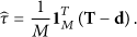
where the fact that the TOA measurement noise vector n is a zero-mean Gaussian random vector has been applied. Differentiating the cost function in (27) with respect to τ and setting the result to zero yield the ML estimator for the clock bias τ. Mathematically, we have

$$\begin{array}{cc}& \widehat{\tau }=\frac{\mathrm{1}}{M}{\mathbf{1}}_M^T(\mathbf{T}-\mathbf{d}).\end{array}$$

(28)

d is defined in (4) and it is unknown because the true source position p is not available. We replace it with $\widehat{\mathbf{d}}$ that has the same functional form as d except that p has been replaced by Step 1 output $\widehat{\mathbf{p}}$ . Hence, the proposed algorithm estimates the clock bias via

$$\begin{array}{cc}& \widehat{\tau }=\frac{\mathrm{1}}{M}{\mathbf{1}}_M^T(\mathbf{T}-\widehat{\mathbf{d}}).\end{array}$$

(29)

We now summarize the processing required to estimate the source position p and the clock bias τ. The proposed algorithm accomplishes the joint synchronization and source localization task by evaluating sequentially (24), (25), (26), and (29). Note that in computing ${\widehat{\mathbf{\phi }}}_{\mathrm{1}}$ and ${\widehat{\mathbf{\phi }}}_{\mathrm{2}}$ using (24) and (25), the true source position p is needed to produce the weighting matrices ${\mathbf{W}}_{\mathrm{1}}$ and ${\mathbf{W}}_{\mathrm{2}}$ . To bypass these difficulties, when evaluating (24), we first set ${\mathbf{W}}_{\mathrm{1}}$ to be an identity matrix of appropriate dimension and compute ${\widehat{\mathbf{\phi }}}_{\mathrm{1}}$ to find ${\mathbf{\phi }}_{\mathrm{1}}$ . Then, (24) is calculated again with p in ${\mathbf{W}}_{\mathrm{1}}$ being replaced by ${\widehat{\mathbf{\phi }}}_{\mathrm{1}}(\mathrm{1}:\mathrm{2})$ that is just obtained. In evaluating (25), the source position estimate from Stage 1 of Step 1 processing is utilized to generate ${\mathbf{W}}_{\mathrm{2}}$ .

4.1. Performance Analysis

We shall establish the efficiency of the algorithm proposed in the previous subsection under the condition that the TOA measurement noise $n_m$ are sufficiently small. Mathematically, we need to show that the algorithm output, namely the source position estimate $\widehat{\mathbf{p}}$ and the clock bias estimate $\widehat{\tau }$ , is unbiased and their covariance matrices are approximately equal to the corresponding CRLBs, that is,

$$\begin{array}{cc}& \mathrm{cov}\left(\widehat{\mathbf{p}}\right)\approx \text{CRLB}\left(\mathbf{p}\right),\end{array}$$

(30)

$$\begin{array}{cc}& \mathrm{cov}\left(\widehat{\tau }\right)\approx \text{CRLB}\left(\tau \right).\end{array}$$

(31)

$\mathrm{cov}(\widehat{\mathbf{p}})$ is the covariance matrix of $\widehat{\mathbf{p}}$ given under (26) and CRLB $(\mathbf{p})$ is the CRLB of the source position p defined in (6b). The validity of (30) can be verified by following the performance analysis procedure adopted in [34]. The unbiasedness of $\widehat{\mathbf{p}}$ can be shown as follows. The estimation error in $\widehat{\mathbf{p}}$ can be written as, from the definitions of $\mathrm{\Delta }\widehat{\mathbf{p}}$ , $\mathrm{\Delta }{\widehat{\mathbf{\phi }}}_{\mathrm{2}}$ and $\mathrm{\Delta }{\widehat{\mathbf{\phi }}}_{\mathrm{1}}$ given below (26), (25), and (24),

$$\begin{array}{cc}& \mathrm{\Delta }\widehat{\mathbf{p}}=\underset{\mathbf{U}}{\underbrace{{\mathbf{B}}_{\mathrm{3}}^{-T}{\left({\mathbf{G}}_{\mathrm{2}}^T{\mathbf{W}}_{\mathrm{2}}{\mathbf{G}}_{\mathrm{2}}\right)}^{-\mathrm{1}}{\mathbf{G}}_{\mathrm{2}}^T{\mathbf{W}}_{\mathrm{2}}{\mathbf{B}}_{\mathrm{2}}{\left({\mathbf{G}}_{\mathrm{1}}^T{\text{W}}_{\mathrm{1}}{\mathbf{G}}_{\mathrm{1}}\right)}^{-\mathrm{1}}{\mathbf{G}}_{\mathrm{1}}^T{\mathbf{W}}_{\mathrm{1}}{\mathbf{B}}_{\mathrm{1}}}}\mathrm{\Delta }\mathbf{r}\mathbf{,}\end{array}$$

(32)

where $\mathrm{\Delta }\mathbf{r}$ is the error in the TDOA measurement vector produced from the TOA measurements $T_m$ , which is defined in (23) and shown to have zero mean. Under the small TOA measurement noise condition, we can ignore the noise in ${\mathbf{G}}_{\mathrm{1}}$ and as a result, $\mathrm{\Delta }\widehat{\mathbf{p}}$ is linearly proportional to $\mathrm{\Delta }\mathbf{r}$ and is zero-mean, which establishes that the source location estimate from the proposed algorithm is unbiased.

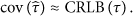
We proceed to prove (31), where $\mathrm{cov}(\widehat{\tau })$ is the covariance matrix of the clock bias estimate in (29) and CRLB $(\tau )$ is the CRLB defined in (6a). As pointed out above (29), the clock bias is identified within the proposed algorithm using an ML estimator. We have shown above that the source position estimate $\widehat{\mathbf{p}}$ is an efficient estimate and as such, it can be expected from the property of the ML estimator [35] that the clock bias estimate $\widehat{\tau }$ would have an accuracy approximately equal to its CRLB. To derive $\mathrm{cov}(\widehat{\tau })$ , the estimation error in $\widehat{\tau }$ , denoted by $\mathrm{\Delta }\widehat{\tau }$ , needs to be found. For this purpose, we expand $\widehat{\mathbf{d}}$ in (29) at the true source position p using the Taylor-series expansion up to the linear term, substitute (4), and subtract τ from both sides of (29) to arrive at

$$\begin{array}{cc}& \mathrm{\Delta }\widehat{\tau }\approx \frac{\mathrm{1}}{M}{\mathbf{1}}_M^T(\mathbf{n}-\mathbf{H}\mathrm{\Delta }\widehat{\mathbf{p}}),\end{array}$$

(33)

where H is defined in (7). It can be shown by putting (32) into (33) that the clock bias estimate $\widehat{\tau }$ from the proposed algorithm is also zero-mean since its estimation error $\mathrm{\Delta }\widehat{\tau }$ is linearly proportional to the zero-mean TOA measurement noise vector n, under small TOA noise condition.

$\mathrm{cov}(\widehat{\tau })$ can be obtained via squaring both sides of (33) and taking expectation. We have, after some simplifications,

$$\begin{array}{cc}& \mathrm{cov}\left(\widehat{\tau }\right)\approx \frac{\mathrm{1}}{M^{\mathrm{2}}}{\mathbf{1}}_M^T\left({\sigma }_n^{\mathrm{2}}{\mathbf{I}}_M+\mathbf{H}\text{CRLB}\left(\mathbf{p}\right){\mathbf{H}}^T-\mathbf{F}-{\mathbf{F}}^T\right){\mathbf{1}}_M,\end{array}$$

(34)

where (30) has been substituted and $\mathbf{F}=\mathbf{H}·\text{E}[\mathrm{\Delta }\widehat{\mathbf{p}}{\mathbf{n}}^T]$ . We shall show that $\mathbf{F}·{\mathbf{1}}_M={\mathbf{0}}_M$ , where ${\mathbf{0}}_M$ is an $M\times \mathrm{1}$ vector of zeros. In particular, after putting (32) and (23),

$$\begin{array}{lll}\mathbf{F}\cdot {\mathbf{1}}_M\hfill & \approx \hfill & \mathbf{H}\mathbf{U}\cdot \text{E}[\Delta \mathbf{r}{\mathbf{n}}^T]{\mathbf{1}}_M\hfill \\ \hfill & =\hfill & \mathbf{H}\mathbf{U}\cdot [-{\mathbf{1}}_{M-1}\hspace{0.17em}\hspace{0.17em}{\mathbf{I}}_{M-1}]{\mathbf{1}}_M={\mathbf{0}}_M.\hfill \end{array}$$

(35)

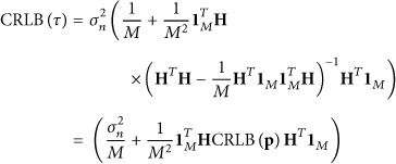
Putting the above result into (34) and comparing (34) with (6a) after applying the matrix inversion lemma [33] and ${\sum }_{m=\mathrm{1}}^M‍{\mathit{\rho }}_{\mathbf{p},{\mathbf{p}}_m}^T={\mathbf{1}}_M^T\mathbf{H}$ , which is

$$\begin{array}{lll}\text{CRLB}(\tau )\hfill & =\hfill & {\sigma }_n^2(\frac{1}{M}+\frac{1}{M^2}{\mathbf{1}}_M^T\mathbf{H}\hfill \\ \hfill & \hfill & \times {\left({\mathbf{H}}^T\mathbf{H}-\frac{1}{M}{\mathbf{H}}^T{\mathbf{1}}_M{\mathbf{1}}_M^T\mathbf{H}\right)}^{-1}{\mathbf{H}}^T{\mathbf{1}}_M)\hfill \\ \hfill & =\hfill & \left(\frac{{\sigma }_n^2}{M}+\frac{1}{M^2}{\mathbf{1}}_M^T\mathbf{H}\text{CRLB}(\mathbf{p}){\mathbf{H}}^T{\mathbf{1}}_M\right)\hfill \end{array}$$

(36)

would yield (31). This completes the establishment of the efficiency of the proposed algorithm.

5. Simulations

We shall demonstrate the estimation performance of the algorithm developed in the previous section for identifying the position and the clock bias of the unknown source in a twostep manner via computer simulations. The simulation scenario is the same as in Section 3.1, which is depicted in Figure 1.

The newly proposed algorithm in Section 4 is applied to estimate the source position p as well as the clock bias fixed at $\tau =\mathrm{15}$  m. The accuracy for source localization and synchronization is quantified using $(\mathrm{1}/L){\sum }_{l=\mathrm{1}}^L{\parallel {\mathbf{p}}_l-\mathbf{p}\parallel }^{\mathrm{2}}$ and $(\mathrm{1}/L){\sum }_{l=\mathrm{1}}^L{\parallel {\tau }_l-\tau \parallel }^{\mathrm{2}}$ , where $L=\mathrm{20,000}$ is the total number of ensemble runs and ${\mathbf{p}}_l$ and ${\tau }_l$ are the source position and clock bias estimates in ensemble l. In each ensemble run, the erroneous TOA measurements are produced by adding to the true values zero-mean Gaussian noise with variance ${\sigma }_n^{\mathrm{2}}$ . For the purpose of comparison, we also realize the algorithm developed in [21] for joint source localization and synchronization.

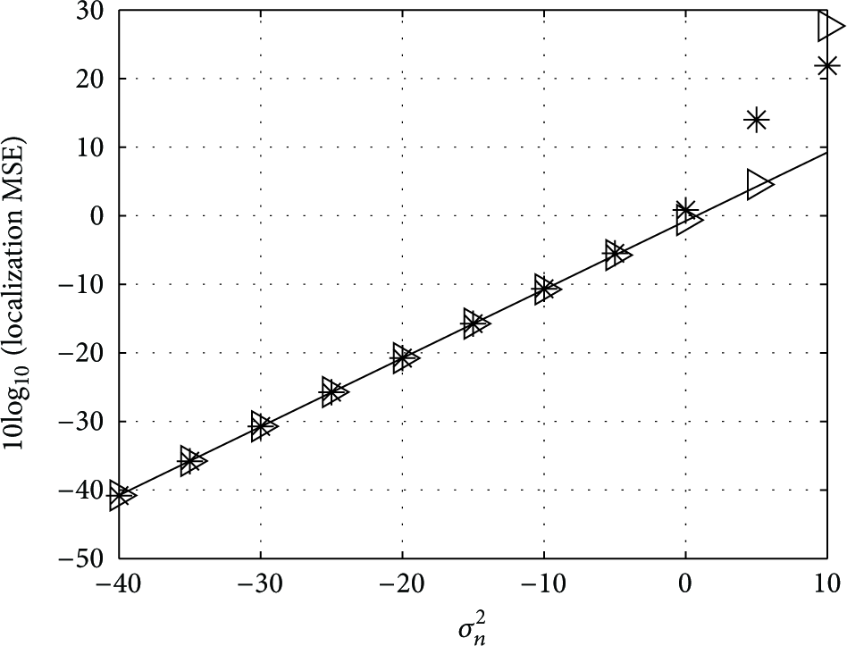
For each of the two sources shown in Figure 1, we generate two figures for plotting the synchronization and source localization MSEs as function of the TOA measurement noise power ${\sigma }_n^{\mathrm{2}}$ , respectively. The corresponding CRLBs, specifically CRLB $(\tau )$ and CRLB $(\mathbf{p})$ from (6a) and (6b), are included in the figures as performance benchmark.

Figures 4 and 5 plot the clock bias and source position estimation MSEs for the source $\mathbf{p}=[\mathrm{50,50}{]}^T$ outside the sensor array. It can be seen from the figures that the proposed algorithm is able to attain the CRLB accuracy for the source position and clock bias before the TOA measurement noise power ${\sigma }_n^{\mathrm{2}}$ reaches $\mathrm{0}$ in log scale. This is consistent with the theoretical performance analysis presented in Section 4.1 that the proposed algorithm is approximately efficient for accurate TOA measurements. On the other hand, the previously developed method from [21] cannot reach the CRLB accuracy, and its synchronization and localization MSEs are higher than the CRLB by an amount of more than 17 dB when ${\sigma }_n^{\mathrm{2}}$ lies in the range from −40 to −25 in log scale. As the TOA measurement noise power further increases over −10 in log scale, the performance improvement due to the use of the newly proposed method is even more significant.

Figure 4

Synchronization accuracy for the source outside the sensor array. Solid line: $\mathrm{tr}(\text{CRLB}(\tau ))$ from (6a), star symbol: synchronization MSE from the proposed method, right triangle symbol: synchronization MSE from the algorithm in [21].

Figure 5

Localization accuracy for the source outside the sensor array. Solid line: $\mathrm{tr}(\text{CRLB}(\mathbf{p}))$ from (6b), star symbol: source localization MSE from the proposed method, right triangle symbol: source localization MSE from the algorithm in [21].

Figures 6 and 7 depict the estimation MSEs for the clock bias and the position of the source $\mathbf{p}=[-\mathrm{10,10}{]}^T$ inside the sensor array. Comparing with Figures 4 and 5 immediately reveals that the estimation performance is much better in this case, mainly because the localization geometry is improved. Moreover, in contrast to the case where the source is outside the sensor array, the proposed method and the algorithm from [21] yield similar estimation accuracy that matches the CRLBs for both the clock bias and the source position. This again verifies the performance analysis results in Section 4.1 on the approximate efficiency of the proposed solution. Interestingly, the method from [21] suffers from the threshold effect later than the new algorithm in this simulation. However, its better performance does not persist as the source location moves outsides the sensor array, as shown in Figures 4 and 5. In contrast, the proposed algorithm can attain the CRLB performance for both cases where the source lies within and outside the sensor array, when the TOA measurement noise power is not sufficiently large.

Figure 6

Synchronization accuracy for the source inside the sensor array. Solid line: $\mathrm{tr}(\text{CRLB}(\tau ))$ from (6a), star symbol: synchronization MSE from the proposed method, right triangle symbol: synchronization MSE from the algorithm in [21].

Figure 7

Localization accuracy for the source inside the sensor array. Solid line: $\mathrm{tr}(\text{CRLB}(\mathbf{p}))$ from (6b), star symbol: source localization MSE from the proposed method, right triangle symbol: source localization MSE from the algorithm in [21].

6. Conclusions and Future Work

In this paper, the TOA-based joint synchronization and source localization problem was considered. Effects of neglecting the presence of the source clock bias in TOA measurements on source location estimation accuracy was first investigated. For this purpose, an MSE analysis was performed for the case where the source is localized via TOA positioning when assuming the source clock bias does not exist, but in fact it is nonzero. Comparing the obtained source localization MSE with that from joint estimating the source position and clock bias, we derived a condition under which ignoring the source clock bias may provide a smaller localization MSE. Numerical examples were provided to validate the analysis and reveal that, in some cases, neglecting the clock bias can severely degrade the localization performance. As a result, a new efficient closed-form solution for joint synchronization and source localization was proposed. The new method can identify the source location and clock bias using a twostep approach. Theoretical performance analysis and simulations were conducted to show that it can achieve the CRLB accuracy for both source location and clock bias estimates under small Gaussian TOA measurement noise.

Some recent work such as [22] adopted a more completed model where both the time offset (clock bias) and skew are considered. However, the proposed least squares (LS) estimator in [22] cannot reach the CRLB accuracy. As a future topic, we would like to derive an efficient closed-form estimator for joint synchronization and source localization in the presence of time skew.