A VANET-Based A* Route Planning Algorithm for Travelling Time- and Energy-Efficient GPS Navigation App

Abstract

Most current navigation devices or apps, based on the global positioning system (GPS), only adopt static information for route planning. Although some are equipped with an RDS-TMC receiver to receive real-time traffic events, many of these real-time traffic events are irrelevant to the vehicle. This paper offers three major contributions. First, a vehicular-ad-hoc-network- (VANET-) based ${\mathrm{\text{A}}}^{\mathrm{*}}$ ( ${\mathrm{\text{VBA}}}^{\mathrm{*}}$ ) route planning algorithm is proposed to calculate the route with the shortest travelling time or the lowest fuel consumption, depending on two real-time traffic information sources, which have not been used in traditional GPS navigation applications. The first traffic information source is the recorded traffic information of the road segment that the vehicle has passed through. It is further exchanged between vehicles through an IEEE 802.11p wireless link. The second traffic information is provided by Google Maps. A GPS navigation app is then implemented on the Android platform to realize ${\mathrm{\text{VBA}}}^{\mathrm{*}}$ . Finally, simulations for six route planning algorithms are executed by VANET simulator The ONE, in one congested and one noncongested time period, respectively. In summary, ${\mathrm{\text{VBA}}}^{\mathrm{*}}$ achieves significant reductions in both the average travelling time and fuel consumption of the planned route, as compared to traditional route planning algorithms.

1. Introduction

As the accuracy of the Global Positioning System (GPS) [1] has improved to within a few meters, GPS applications have become increasingly popular in our daily lives. Of these applications, the GPS navigation system is one of the most used. Before the development of GPS navigation systems, people had to use paper maps for travel directions. However, with the aid of voice-activated GPS navigation systems, people can now plan their routes on an electronic map in real time to help them reach their destinations efficiently and smartly.

However, if the electronic map information is out of date, or if a traffic incident or road maintenance event occurs in real time, the GPS navigation system may plan an erroneous route. In recent years, many methods for addressing this problem have been developed, including real-time online road information supported by the Radio Data System-Traffic Message Channel (RDS-TMC) [2], which uses FM channels to transfer real-time traffic data to vehicles. However, most traffic data provided by RDS-TMC are for specific roads in urban areas or highways. Thus, on-board GPS navigation systems may not receive useful road information from RDS-TMC to assist in route planning. Furthermore, due to RDS-TMC's low bit rate, it is not possible to transfer large amounts of traffic data to vehicles with acceptable delays. On the current market, GPS navigation apps such as Garmin StreetPilot Onboard [3] for Apple iPhone/iPad or PaPaGo! Mobile [4] for the Android platform are becoming more and more prevalent. Offline maps are preloaded in these apps for the user to look up addresses and millions of points of interest (POIs), such as gas stations, restaurants, and parking lots, without wireless coverage. Moreover, if a wireless connection is available, these apps can retrieve real-time road and traffic information from the Internet to plan a faster route to the destination by avoiding roads under construction or congestion. However, they exhibit problems similar to those of RDS-TMC, that is, not all roads have real-time information, and the wireless connection to the Internet is a must.

As an alternative communication technology for exchanging real-time information by long-range 3G/4G, IEEE 802.11p, and so forth, WAVE architecture [5] has been designed for short-range vehicle-to-vehicle (V2V) communication. When people drive on the road, these vehicles can transfer information to each other through a dynamically formed vehicular ad hoc network (VANET) [6]. If a vehicle has encountered a traffic incident, it can send safety messages to warn neighboring vehicles with information including the time, location, and status of the incident [6, 7]. These neighboring cars then further forward the safety messages to their neighbors, such that they can replan their routes in real time to avoid encountering the incident. In this way, the travelling time and fuel consumption, that is, travelling costs, of vehicles can be reduced. On the other hand, the Dijkstra shortest path [8] and A-star ( ${\text{A}}^{*}$ ) [9] algorithms are usually used to plan routes in GPS navigation systems. Compared to Dijkstra, ${\text{A}}^{*}$ achieves shorter computation time by using heuristic functions. It uses a best-first search and finds a least-cost path from a given initial node to one destination node with lower hardware requirements. Recent studies [10, 11] have therefore extended ${\text{A}}^{*}$ into new path planning strategies. However, these traditional route planning algorithms use static information such as the speed limit, instead of the real-time speed of each road segment, to calculate the route to the destination, which usually underestimates the actual travelling time and fuel consumption in turn. Therefore, dynamic route planning schemes, which incorporate real-time traffic information and react to the dynamic conditions of the road, are more robust than static ones for congestion alleviation [12].

This paper focuses on designing and implementing an Android-based navigation app, which has the following advantages for reducing the travelling time, fuel consumption, and emitted carbon dioxide, for dynamic route planning.

• (1)

A generic format to record the vehicle's driving information on an Android platform like a smart phone or tablet PC carried by the vehicle's driver is designed. This information includes the time spent, fuel consumed, and average speed on each road segment that the vehicle has passed through recently.

(2)

Each vehicle will distribute its recorded driving information to its neighboring vehicles in the VANET, which means that these vehicles are within the IEEE 802.11p wireless communication range. Thus, each vehicle may be notified of actual traffic information of road segments, which it has not known, by its neighboring vehicles. As more dynamic road information is received from other vehicles, each vehicle can estimate future road information more accurately. In this way, the kind of dynamic route planning algorithm executed in the Android platform of each vehicle can output a more precise path to the destination than traditional static algorithms do.

(3)

The real-time traffic data of road segments accessible from Google Maps [13] is used in this Android-based GPS navigation app to compensate for the road information missed in the dynamic road information received from neighboring vehicles. With these two kinds of road information, this Android-based GPS navigation app can more accurately estimate future road information by the exponentially weighted moving average (EWMA) function [14] modified in this paper.

(4)

Using the two kinds of road information previously mentioned, an improved ${\text{A}}^{*}$ route planning algorithm, that is, the VANET-based ${\text{A}}^{*}$ ( $\text{VB}{\text{A}}^{*}$ ), is proposed to calculate an initial route when the vehicle starts its GPS navigation. Two criteria are adopted in this improved algorithm to plan the route with the shortest travelling time and the lowest fuel consumption, respectively. Whenever the vehicle has received newer road information from neighboring vehicles or Google Maps, this $\text{VB}{\text{A}}^{*}$ algorithm will recalculate the route to the destination and update the visual and auditory guidance information for the driver in real-time.

The remainder of this paper is organized as follows. Traditional route planning methods and Android-based navigation systems are discussed in Section 2. Section 3 explains detailed app design, including real-time road information collection and distribution mechanisms through the VANET, of the $\text{VB}{\text{A}}^{*}$ route planning algorithm. In Section 4, implementation issues and screen snapshots of this GPS navigation app on the Android platform are presented. After this, we present simulation results to exhibit the significant performance improvements of the $\text{VB}{\text{A}}^{*}$ algorithm reducing travelling time and fuel consumption. Finally, Section 6 concludes this paper.

2. Related Work

2.1. Route Planning Strategy

The shortest path problem is based on graph theory. It is a problem for a graph with nodes and arcs to find the shortest path between two nodes. The Dijkstra and ${\text{A}}^{*}$ algorithms are usually used to solve it. The Dijkstra algorithm can find the shortest path from a particular node to other nodes with time complexity $O(n^2)$ , where n is the number of nodes. Its key idea is to construct a spanning tree of minimum total length from the starting node to all other nodes recursively. This algorithm is often used as a benchmark solution for comparison with other routing algorithms. In the following, the concepts of ${\text{A}}^{*}$ and its extensions are discussed.

The ${\text{A}}^{*}$ route planning algorithm uses the best-first search (BFS) [9] to find the shortest path in the graph. As ${\text{A}}^{*}$ traverses the graph, it follows the path of the lowest known heuristic cost, keeping a sorted priority queue of alternate path segments. It uses the heuristic function $F(n)$ , formulated as (1), to determine the order in which the BFS visits nodes and then to calculate the total cost of each path:

$$\begin{array}{cc}& F\left(n\right)=G\left(n\right)+H\left(n\right),\end{array}$$

(1)

where $G(n)$ represents the cost from the starting node to current node n in the graph, and $H(n)$ represents the heuristic estimate of the cost from the current node n to the destination node. If the cost is measured by the distance between two nodes, the straight-line distance from node n to the destination is usually used as $H(n)$ .

As shown in Figure 1, if the angle θ between the neighbor road of the current node, that is, an intersection in this paper, and the straight line between the current node and the destination node is smaller, it means that the direction of the neighbor road is closer to the straight line to the destination, which is used as $H(n)$ as previously mentioned. Thus, the extended ${\text{A}}^{*}$ algorithm in [15] modifies the original ${\text{A}}^{*}$ heuristic function by multiplying an angle function $A(n)$ as (2), where $A(n)$ is formulated as (3). The smaller the angle is, the smaller the values of $A(n)$ and $F(n)$ , that is, the estimated total cost of the path, will be. Therefore, this modification prefers to choose the neighbor road with the smaller θ, which in turn finds the lowest cost path more quickly than does the original ${\text{A}}^{*}$ :

$$\begin{array}{cc}& F\left(n\right)=A\left(n\right)\times \left(G\left(n\right)+H\left(n\right)\right),\end{array}$$

(2)

$$\begin{array}{cc}& A\left(n\right)=1-\mathrm{\hspace{0.17em}\hspace{0.17em}}\frac{180-\theta }{180+\theta }.\end{array}$$

(3)

Figure 1

The angle between the neighbor road segment and the straight line to the destination node.

The second improvement of the ${\text{A}}^{*}$ heuristic function in [15] is to consider the dynamic road speeds by modifying $F(n)$ as (4), where $G(n)$ and $H(n)$ are multiplied by their corresponding weighting parameters, that is, $W_n(n)$ and $W_{n+1}(n)$ , respectively. $W_n(n)$ is calculated by (5), where $S_n$ and $S_{na}$ denote the average driving speed and the highest speed limit of all road segments from the starting node to current node n, respectively. Similarly, $W_{n+1}(n)$ is calculated by (6), where $S_{n+1}\mathrm{\hspace{0.17em}\hspace{0.17em}}$ and $S_{n+1a}$ denote the average driving speed and the average speed limit of all road segments from current node n to each neighbor node of n, respectively. Thus, larger $S_n$ and $S_{n+1}$ , that is, higher average driving speeds of all road segments from the starting node to current node n and from current node n to each neighbor node of n, will produce smaller $W_n(n)$ and $W_{n+1}(n)$ , which in turn generates smaller $F(n)$ :

$$\begin{array}{cc}& F\left(n\right)=A\left(n\right)\left(G\left(n\right)\times W_n\left(n\right)+H\left(n\right)\times W_{n+1}\left(n\right)\right),\end{array}$$

(4)

$$\begin{array}{cc}& W_n\left(n\right)=\{\begin{array}{cc}1-\left|\frac{S_{na}-S_n}{S_{na}+S_n}\right|,\hfill & S_{na}<S_n\hfill \\ 1,\hfill & S_{na}=S_n\hfill \\ 1+\left|\frac{S_{na}-S_n}{S_{na}+S_n}\right|,\hfill & S_{na}>S_n,\hfill \end{array}\mathrm{\hspace{0.17em}\hspace{0.17em}}\mathrm{\hspace{0.17em}\hspace{0.17em}}\end{array}$$

(5)

$$\begin{array}{cc}& W_{n+1}\left(n\right)=\{\begin{array}{cc}1-\left|\frac{S_{n+1a}-S_{n+1}}{S_{n+1a}+S_{n+1}}\right|,\hfill & S_{n+1a}<S_{n+1}\hfill \\ 1,\hfill & S_{n+1a}=S_{n+1}\hfill \\ 1+\left|\frac{S_{n+1a}-S_{n+1}}{S_{n+1a}+S_{n+1}}\right|,\hfill & S_{n+1a}>S_{n+1}.\hfill \end{array}\end{array}$$

(6)

2.2. Existing GPS Navigation and Route Sharing Systems

Most GPS navigation systems on the market provide users with an offline map and several modes for planning their routes. Some can receive RDS-TMC real-time traffic information for planning a route that does not pass through a congested area. One famous Android-based GPS navigation app is the Garmin StreetPilot [3], which is able to plan a route with the shortest distance and time modes. It can access real-time traffic information, photoLive traffic cameras, and fuel pricing as optional services. Recently, Garmin introduced ecoRoute energy-saving assistant [16] for calculating a more fuel-efficient route and tracking fuel usage. By entering the fuel type, cost, and consumption at low and high driving speeds, the driver can check information on driving distance, driving time, average fuel consumption, cost of fuel used, carbon footprint, and so forth. It also can help the driver become more fuel-efficient by letting them know if they are driving efficiently. Like Garmin StreetPilot, PAPAGO! Mobile [4] also provides many route planning modes and can update its electronic map automatically via WiFi or 3G.

On the other hand, several researches have studied the issue of sharing route information among vehicles. In [17], the authors proposed a route information sharing mechanism to inform the route information server of forthcoming route details. Based on routes collected from the server, each driver can change their route to reduce traffic congestion. However, this sharing was assumed to be achieved through cellular communication with a remote and centralized route information server. It is obvious that this server is the performance bottleneck and the single point of failure. Furthermore, significant latencies are incurred in transferring the huge amount of route information between the vehicles and the route information server. As an alternative, a peer-to-peer VANET application for sharing and exchanging road traffic information for vehicles to detect and avoid traffic congestion was presented in [18]. A pull-based geocast protocol was also designed for vehicles to cooperatively collect and disseminate data. However, this work adopted the time-consuming Dijkstra algorithm to find the least congested route to a given destination according to the congestion index of each road segment that the vehicle had driven through. Moreover, the least congested route found might not necessarily be the one with the shortest travelling time or the lowest fuel consumption, which are two important criteria in the proposed ${\text{VBA}}^{*}$ for planning a time- or energy-efficient route for the ecofriendly lifestyle. In summary, all navigation systems or apps allow users to choose different modes to plan their routes on an off-line electronic map. Without the ability to access real-time traffic information through wireless connections, most cannot help drivers avoid congested areas so as to reduce the travelling time, cost of fuel, and carbon emissions. However, with the proposed ${\text{VBA}}^{*}$ algorithm, which can plan the shortest travelling time or the lowest fuel cost routes in terms of real-time traffic information exchanged between neighboring vehicles via VANET, the Android-based GPS navigation app designed and implemented in this paper can overcome this defect.

3. System Design

In this section, the format for recording the vehicle's driving information, the mechanism to distribute real-time traffic information among contacted vehicles through the VANET, and the flow to estimate the real-time traffic information of next time zone are first described. Then, based on the traffic information distributed among vehicles and accessed from Google Maps, two versions of the modified ${\text{VBA}}^{*}$ route planning algorithms are proposed for meeting the shortest travelling time and the lowest fuel consumption criteria.

3.1. The VANET-Based Traffic Information Distribution and Estimation

3.1.1. Two Traffic Information Sources

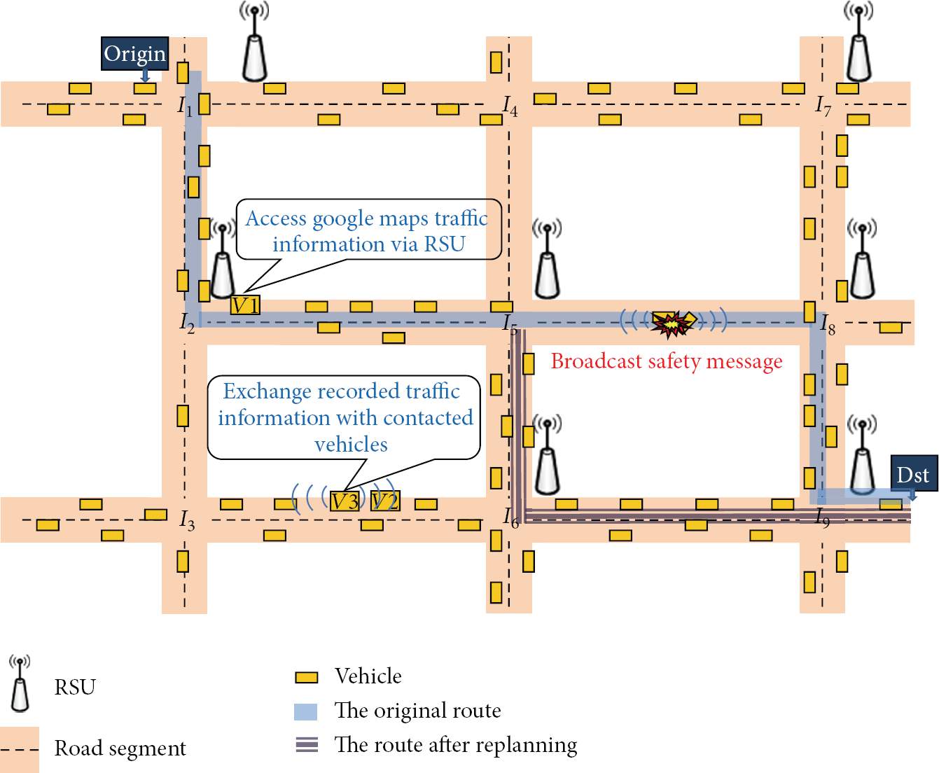
The network topology for the proposed ${\text{VBA}}^{*}$ to plan routes with the shortest travelling time and the lowest fuel consumption is shown in Figure 2. In VANET, the roadside unit (RSU) acts as a wireless LAN access point and enables vehicles within its wireless transmission range to communicate with devices in the network infrastructure. There are two traffic information sources in this paper. The first is the on-board GPS device and the electronic road database, allowing the vehicle to identify its current GPS location and record information such as the instantaneous driving speed in its memory when the vehicle starts to drive on the road. According to the traffic information recording flow shown in Figure 3, the vehicle's on-board GPS device detects whether it has passed through an intersection, which indicates an end of the road segment. If it has, all recorded driving speeds are averaged and stored in the AverageSpeed field of the three-field format for traffic information of this road segment, as listed in Table 1, with correct values in the RoadSegmentID and RecordTime fields, which specify the time the vehicle leaves this road segment.

Table 1

The three-field format for traffic information of a road segment.

Field name	Description
Road segment ID	The unique ID of the road segment between two adjacent intersections. For example, a road segment in Shimin Blvd, Taipei, Taiwan is tagged with 6300009004232 as its ID [19]
Record time	The time at which traffic information is recorded
Average speed	The average driving speed of this road segment

Figure 2

Network topology for the proposed ${\text{VBA}}^{*}$ .

Figure 3

The traffic information recording flow of the vehicle.

As a vehicle like vehicle V1 in Figure 2 drives into the wireless communication range of an RSU, it can access the real-time and historic traffic information from Google Maps as the second source via the RSU. Google Maps divides an hour into 4 time zones, and each time zone lasts for 15 minutes. As shown in Figure 4, four different colors are used to represent four different driving speeds. The road segment colored in green, yellow, red, or red-black means that its driving speed is fast, modest, slow, or congested, respectively. However, Google Maps does not provide traffic information on all road segments, but only on major roads in urban areas or highways. Therefore, the Google Maps information is combined with the following proposed VANET traffic information distribution mechanism, and these two traffic sources are aggregated to supply much more traffic information for the ${\text{VBA}}^{*}$ route planning algorithm, which will be described later. As a result, the planned ${\text{VBA}}^{*}$ route is more accurate and reliable for driving navigation than traditionally planned routes.

Figure 4

Real-time traffic information on Google Maps.

3.1.2. The Traffic Information Distribution Mechanism through the VANET

As previously mentioned, the vehicle continuously collects traffic information as it drives on the road. Whenever another vehicle enters the IEEE 802.11p transmission range of another vehicle, for example, as vehicle V2 in Figure 2 contacts V3, the VANET-based traffic information distribution mechanism proposed in this paper is activated. As shown in Figure 5, by exchanging IEEE 802.11p frames that contain the collected traffic information in the format listed in Table 1 for recent time zones of each road segment that the vehicle has passed through with neighbor vehicles, each vehicle can be notified of the historic traffic information of the road segments it may not have driven through.

Figure 5

The traffic information distribution flow.

3.1.3. Traffic Information Estimation of the Next Time Zone

As soon as the vehicle driver intends to plan a route from its origin to destination with the proposed ${\text{VBA}}^{*}$ algorithm, as shown in Figure 2, the traffic information, that is, the driving speed, of the next time zone for each road segment should first be estimated, with the flow shown in Figure 6. The recorded traffic information is classified into the corresponding 15-minute time zone, according to the time zone diagram of Google Maps shown in Figure 7. Then, the average recorded driving speed of the road segment for each time zone is calculated. 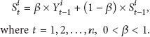If Google Maps provides historic traffic information for a road segment that has already had its average recorded driving speed calculated, these two values, that is, the average recorded driving speed and the speed retrieved from Google Maps, are averaged by a weighting factor α to represent the observed driving speed of each time zone for a road segment, which is formulated by (7), where $A_t^i$ , $G_t^i$ , and $Y_t^i$ denote the average recorded driving speed, the speed retrieved from Google Maps, and the observed driving speed of time zone t for road segment i, respectively:

$$\begin{array}{cc}& Y_t^i=\alpha \times A_t^i+\left(1-\alpha \right)\times G_t^i,\hspace{1em}\text{where}\mathrm{\hspace{0.17em}\hspace{0.17em}}0\le \alpha \le 1.\end{array}$$

(7)

Figure 6

The flow to estimate traffic information of the next time zone.

Figure 7

The time zone diagram of Google Maps.

After this, the driving speed $S_t^i$ of the next time zone t for road segment i can be estimated by the EWMA function [14], which is formulated in (8), where β is the weighting factor and $S_{t-1}^i$ and $Y_{t-1}^i$ denote the estimated and observed driving speeds of time zone $t-1$ for road segment i, respectively. With the EWMA, less weight is given to the driving speed of older time zones, and greater weight is given to that of more recent ones. Finally, the estimated driving speed $S_t^i$ of the next time zone t for road segment i is recorded and used in the following ${\text{VBA}}^{*}$ route planning algorithm:

$$\begin{array}{l}\phantom{00}{S}_t^i=\beta \times Y_{t-1}^i+\left(1-\beta \right)\times S_{t-1}^i,\\ \text{where}\hspace{0.17em}\hspace{0.17em}t=1,2,\dots ,n,\hspace{0.17em}\hspace{0.17em}0<\beta <1.\end{array}$$

(8)

3.2. The VBA* Route Planning Algorithm

In this paper, we will improve the heuristic function of the ${\text{A}}^{*}$ route planning algorithm with two planning criteria, that is, the shortest travelling time and the lowest fuel consumption, to find the path from the starting location, that is, origin, to the destination of the vehicle, respectively. Each road segment from the road database provided by the Institute of Transportation, MOTC, Taiwan, [19] contains its road identification (ID), name, direction, and longitude and latitude coordinate values of its two ends, that is, intersections with adjacent road segments. With coordinate values of both ends, the length of each road segment can be calculated. According to the historic driving speed accessed from Google Maps and those exchanged with neighboring vehicles, the vehicle driving speed $S_t^i$ of the next time zone t on road segment i can be estimated by the EWMA equation, as previously described.

3.2.1. VBA* with the Shortest Travelling Time Criterion

In the following, the term “node” is used to represent the end, that is, an intersection, of a road segment. Equation (9) is used as the improved $\text{VB}{\text{A}}^{*}$ to meet the shortest travelling time criterion. There are two modifications in $\text{VB}{\text{A}}^{*}$ . First, as shown in Figure 8, $G(n)$ in the original ${\text{A}}^{*}$ is replaced by the sum of the travelling time of each road segment that the vehicle has passed through when it has reached the current node n. The travelling time of road segment i is calculated by dividing its length $L^i$ over its average driving speed $S_t^i$ for time zone t, as shown in (9). Second, the heuristic function $H(n)$ in the original ${\text{A}}^{*}$ is replaced by the second term of (9) to find a neighbor node that has the minimal value among all neighbor nodes of current node n. $H(n)$ denotes the straight-line distance from node n to the destination, $S_t^n$ is the estimated driving speed of the next road segment from current node n to its neighbor node $n+1$ , and ${\theta }_t^n$ ( $0^{°}\le {\theta }_t^n\le {180}^{°}$ ) is the angle between the next road segment from current node n to its neighbor node $n+1$ and the straight line from node n to the destination. Because there may not be a next road segment that has the same direction as the straight line of $H(n)$ , that is, ${\theta }_t^n=0^{°}$ , we adopt $\cos {\theta }_t^n$ as the denominator of the second term to find the smallest angle between the next road segment and the straight line of $H(n)$ . For example, as shown in Figure 7, angles between the next road segment from current node n to three neighbor nodes ${(n+1)}^1$ , ${(n+1)}^2$ , and ${(n+1)}^3$ and the straight line are ${\theta }_1$ , ${\theta }_2$ , and ${\theta }_3$ , respectively. Because the range of the angle is $[0^{°},{180}^{°}]$ , the range of its cosine value is $[1,-1]$ . The smaller the angle is, the larger the cosine value of the angle will be. Therefore, a smaller angle in turn produces a smaller value for the second term. Because ${\text{A}}^{*}$ and the improved $\text{VB}{\text{A}}^{*}$ cannot handle negative cost, we simply use $(2+\cos {\theta }_t^n)$ , with a range of $[\mathrm{3,1}]$ , to ensure that the denominator of the second term is greater than 0:

$$\begin{array}{cc}& F\left(n\right)=\sum _{i=0}^{n-1}\frac{L^i}{S_t^i}+\frac{H\left(n\right)}{S_t^n\times \left(2+\cos {\theta }_t^n\right)}.\end{array}$$

(9)

Figure 8

The angle between the next road segment from the current node n to its neighbor node $n+1$ and the straight line from node n to the destination.

3.2.2. VBA* with the Lowest Fuel Consumption Criterion

To fulfill the lowest fuel consumption criterion, (10) is proposed for the improved ${\text{VBA}}^{*}$ . Similar to two modifications made in (9), the original $G(n)$ is first replaced by the sum of the amount of fuel consumed in each road segment that the vehicle has passed through from the starting node to the current node. The amount of fuel consumed in road segment i is equal to the product of its length $L^i$ and the fuel consumption per kilometer $O(S_t^i)$ , which is a function of its average driving speed $S_t^i$ for time zone t, as shown in Figure 9 [20]. Then, the heuristic function $H(n)$ in the original ${\text{A}}^{*}$ is updated as the second term in (10) to find a neighbor node that has the minimal value, that is, the amount of consumed fuel, for the second term among all neighbor nodes of current node n. In (10), $H(n)$ also denotes the straight-line distance from node n to the destination, $S_t^n$ is the estimated driving speed of the next road segment from current node n to its neighbor node $n+1$ , $O(S_t^n)$ is the fuel consumption per kilometer with the estimated driving speed $S_t^n$ , and ${\theta }_t^n$ ( $0^{°}\le {\theta }_t^n\le {180}^{°}$ ) is the angle between the next road segment and the straight line. To find the next road segment with the smallest angle with the straight line, we also adopt $(2+\cos {\theta }_t^n)$ as the denominator of the second term in (10):

$$\begin{array}{cc}& F\left(n\right)={\sum }_{i=0}^{n-1}\left(L^i\times O\left(S_t^i\right)\right)+\frac{H\left(n\right)\times O\left(S_t^n\right)}{\left(2+\cos {\theta }_t^n\right)}.\end{array}$$

(10)

Figure 9

An example of the relationship between the driving speed and the corresponding fuel consumption per kilometer [20].

Besides the driving speed, many other factors can influence fuel consumption. They include route attributes, personal characteristics, trip characteristics, and environmental conditions [21]. Important fuel mileage tips can help the driver reduce the amount of fuel consumed. For example, keeping an engine properly tuned and tires inflated to the proper pressure can improve the fuel mileage up to 40 and 3.3 percent, respectively [22]. Sensible driving can lower the fuel mileage by 33 percent at highway speeds and by 5 percent around town [23]. Observing the speed limit, avoiding excessive idling, removing excess weight, and using cruise control also improve energy efficiency. On the other hand, aaMOTION in [24] proposed mathematical equations to determine the direct vehicle operating cost by using a cost factor to convert the fuel cost to total running cost including fuel, repair, and maintenance. Authors in [25] argued that excess fuel consumption may be avoided by the development of an optimal driving strategy through reducing aggressive driving and maintaining a steady speed. They considered the optimal driving strategy model as an optimal control problem, which was then formulated as a constrained optimization programming subject to speed profile, energy flows, engine load, combustion products, demand for transport service, and gear ratio selection. Because deriving a precise fuel consumption model is beyond the scope of this paper, please refer to the related work for details. Please also note that the fuel consumption function $O(S_t^i)$ in (10) can be replaced by the newly developed one to estimate fuel consumption more accurately.

4. System Implementation

This time- and energy-efficient Android GPS navigation app is implemented on the Google Android 4.1 platform with Eclipse and Android Development Tools (ADT) [26] that support JAVA 1.7. Its main function is to realize the ${\text{VBA}}^{*}$ algorithm for planning a route to meet one of two criteria, that is, the shortest travelling time and the lowest fuel consumption. Important snapshots of this app are shown in the following.

In order to plan a route from the starting location of the vehicle, that is, the blue pin in Figure 10, its driver first has to choose the destination location, that is, the red pin in Figure 10, and then press the “Planning” button at the upper right corner of the app screen. Therefore, the initial planned route from the starting location to the destination, calculated with the static information of the offline electronic map, is shown as the purple line in Figure 10. Associated information about this route, such as the travelling distance, time, amount of fuel consumed, and the average speed, is listed in the green box by clicking the “Route Information” button. Because no dynamic traffic information is used to calculate this initial route, the estimated information listed in parentheses is the same as the original information.

Figure 10

Information of the initial planned route.

According to (8), Figure 11 shows the estimated traffic information of each road segment in the electronic map, that is, the speed of the next time zone, where each road segment is colored in green, yellow or red to represent the low, normal, or high congestion level, respectively, after the vehicle under navigation has exchanged its recorded traffic information with others. Details of the exchanged traffic information such as the list of road segments and the estimated speed of the chosen road segment can be examined, as shown in Figure 11. If too much information has been exchanged, the driver can use the “search” function to find information on a specific road segment.

Figure 11

Details of the exchanged traffic information.

When the driver chooses the lowest fuel consumption criterion as the route planning option in Figure 12 and clicks the “planning” button again, a new energy-efficient route, drawn as the indigo line in Figure 13, is dynamically replanned by the proposed ${\text{VBA}}^{*}$ algorithm to avoid those congested road segments which would cause the vehicle to consume more fuel. Based on estimated traffic information, new information about this replanned route is shown in the green box. Though this replanned route has a longer travelling distance, it achieves a shorter travelling time, lower fuel consumption and higher driving speed than the original route planned with the static information.

Figure 12

The setup page for route planning options.

Figure 13

The dynamically replanned route based on the exchanged traffic information.

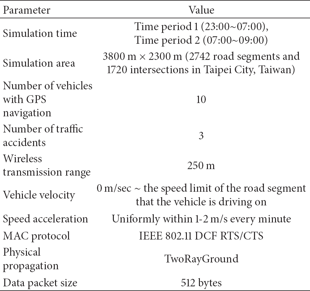
5. Performance Evaluations

5.1. Simulation Environment

In reality, it is hard to execute a large scale evaluation to measure the real travelling distance, time, speed, and consumed fuel of vehicles navigated by this ${\text{VBA}}^{*}$ and other traditional route planning algorithms. We therefore compare simulation results of the travelling distance, time, and fuel consumption for six route planning algorithms: Dijkstra, ${\text{A}}^{*}$ , TTU- ${\text{A}}^{*}$ (angle + speed), TTU- ${\text{A}}^{*}$ (angle), ${\text{VBA}}^{*}$ (Time), and ${\text{VBA}}^{*}$ (Fuel), using the Opportunistic Network Environment (The ONE) simulator [27]. TTU- ${\text{A}}^{*}$ (angle) and TTU- ${\text{A}}^{*}$ (angle + speed), which use (2) and (4), respectively, as described in Section 2, are two extended ${\text{A}}^{*}$ algorithms proposed in [15]. ${\text{VBA}}^{*}$ (Time) and ${\text{VBA}}^{*}$ (Fuel) denote our proposed ${\text{VBA}}^{*}$ algorithms, which satisfy the shortest travelling time and the lowest fuel consumption criteria, respectively. Simulation parameters used are listed in Table 2. As shown in Figure 14, the electronic map used in this simulation contains 2742 road segments and 1720 intersections in Taipei City, Taiwan. Each vehicle follows the IEEE 802.11 MAC protocol with Distributed Coordination Function (DCF) RTS/CTS enabled and the TwoRayGround physical propagation model with a maximal transmission range of 250 m. The initial vehicle distribution follows the realistic vehicle density statistics from the traffic database of the Traffic Engineering Office, Taipei City Government [28]. As listed in Table 3, the urban traffic statuses of four time periods, 07:00~09:00, 12:00~13:00, 17:00~19:00, and 22:00~23:00, in a day are usually considered as congested, but those of the other four periods are noncongested. According to the rule that the driving speed in the congested time period is much lower than the speed limit of the road segment, but that in the noncongested time period, it is closer to the speed limit, average performance results of 10 vehicles executing these six route planning algorithms for 20 runs in one congested time period, time period 1, and one noncongested time period, time period 2, will be compared below. The destination of each vehicle for navigation is uniformly distributed in the map. The initial driving speed of the vehicle when the simulation starts is uniformly generated with the range of $[0,{\text{SL}}_t^i]$ , where ${\text{SL}}_t^i$ denotes the speed limit of road segment i, where the vehicle is initially located when the simulation begins for time period t. The acceleration of the vehicle varies uniformly within ±1-2 m/s every minute. However, the instantaneous speed of every vehicle cannot exceed the speed limit of the road segment it is driving through. As the first type of traffic information in the ${\text{VBA}}^{*}$ algorithm, the observed driving speeds for all time zones of each time period are calculated by averaging those generated driving speeds in each time zone, as previously described. On the other hand, because Google Maps does not provide any formal function to access its traffic information, we have implemented a preprocessing program to retrieve it as the second traffic information source of the ${\text{VBA}}^{*}$ algorithm by matching the drawn street maps of Google Maps with the electronic map used.

Table 2

Simulation parameters.

Parameter	Value
Simulation time	Time period 1 (23:00~07:00), Time period 2 (07:00~09:00)
Simulation area	3800 m × 2300 m (2742 road segments and 1720 intersections in Taipei City, Taiwan)
Number of vehicles with GPS navigation	10
Number of traffic accidents	3
Wireless transmission range	250 m
Vehicle velocity	0 m/sec ~ the speed limit of the road segment that the vehicle is driving on
Speed acceleration	Uniformly within 1-2 m/s every minute
MAC protocol	IEEE 802.11 DCF RTS/CTS
Physical propagation	TwoRayGround
Data packet size	512 bytes

Table 3

Eight time periods in a day.

	Start time	End time	Traffic status
Time period 1	23:00 pm	07:00 am	Noncongested
Time period 2	07:00	09:00	Congested
Time period 3	09:00	12:00	Noncongested
Time period 4	12:00	13:00	Congested
Time period 5	13:00	17:00	Noncongested
Time period 6	17:00	19:00	Congested
Time period 7	19:00	22:00	Noncongested
Time period 8	22:00	23:00	Congested

Figure 14

The electronic map of Taipei City, Taiwan used in this simulation.

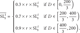
Furthermore, in order to examine the influence of real-time traffic accidents, which result in the dynamic planning of new routes, on the performances of these six algorithms, three traffic accidents are generated for a simulation run in a random position on the map at a random time during the time period. The smaller the straight-line distance between the center of the road segment and the position of the accident, the lower the driving speed of this road segment after the accident will be. In order to add this behavior into our simulation, the new driving speed limit $\stackrel{-}{{\text{SL}}_t^i}$ of road segment i within the distance range D of $[\mathrm{0,200}/3)$ , $[200/\mathrm{3,400}/3)$ , and $[400/\mathrm{3,200})$ meters to the accident position is reduced from ${\text{SL}}_t^i$ to $0.3\times r\times {\text{SL}}_t^i$ , ${0.7\times r\times \text{SL}}_t^i$ , and ${0.9\times r\times \text{SL}}_t^i$ , respectively, as formulated by (11), where ${\text{SL}}_t^i$ denotes the original speed limit of road segment i at time period t when no accident has occurred, and r ( $0\le r\le 1$ ) is the ratio of the new driving speed limit over the original one. In the simulation, values of r are set as 0.2, 0.4, 0.6, and 0.8, respectively:

$$\begin{array}{cc}& \stackrel{-}{{\text{SL}}_t^i}=\{\begin{array}{cc}0.3\times r\times {\text{SL}}_t^i\hfill & \text{if}\mathrm{\hspace{0.17em}\hspace{0.17em}}D\in \left[0,\frac{200}{3}\right)\hfill \\ \hspace{0.17em}\hfill & \hspace{0.17em}\hfill \\ {0.7\times r\times \text{SL}}_t^i\hfill & \text{if}\mathrm{\hspace{0.17em}\hspace{0.17em}}D\in \left[\frac{200}{3},\frac{400}{3}\right)\hfill \\ \hspace{0.17em}\hfill & \hspace{0.17em}\hfill \\ {0.9\times r\times \text{SL}}_t^i\hfill & \text{if}\mathrm{\hspace{0.17em}\hspace{0.17em}}D\in \left[\frac{400}{3},200\right).\hfill \end{array}\end{array}$$

(11)

5.2. Simulation Results

Four performance metrics of six route planning algorithms, that is, the average travelling time, distance, speed, and fuel consumption, are compared below. First, Figures 15 and 16 show the results of their average travelling times with four different r values in Time Periods 1 and 2, respectively. No matter which r value is used in the simulation, the average travelling times of Dijkstra, Original ${\text{A}}^{*}$ , and TTU- ${\text{A}}^{*}$ (angle) are the highest of the six algorithms because their design criteria are focused on finding the route with the shortest travelling distance instead of that with the smallest travelling time. TTU- ${\text{A}}^{*}$ (angle + speed) gives higher weights to road segments with higher driving speeds and smaller angles to the destination, which in turn reduces its travelling time. On the other hand, with the modified heuristic function $H(n)$ for finding a neighbor node that contributes the minimal travelling time to $F(n)$ among all neighbor nodes of current node n in (9), ${\text{VBA}}^{*}$ (time) achieves the smallest average travelling time of all the algorithms. Though the modified $H(n)$ term of ${\text{VBA}}^{*}$ (fuel) in (10) tries to find a neighbor node that has the minimal amount of consumed fuel among all neighbor nodes of current node n, ${\text{VBA}}^{*}$ (fuel) achieves a lower average travelling time than the other four algorithms. This is because the fuel consumption per kilometer is highly dependent on the estimated driving speed of the vehicle; the route found by ${\text{VBA}}^{*}$ (Fuel) with the lowest amount of fuel consumption is the route with the highest driving speed, when the speed is below 79 km/hr as shown in Figure 9. Furthermore, because r is the ratio for reducing the speed limit of the road segment near the accident, a lower r value incurs a lower speed limit after the accident and a higher average travelling time for each algorithm. Finally, the travelling speed on each road segment in time period 1, that is, the noncongested time period, is usually lower than that in time period 2, that is the congested time period. Therefore, the average travelling times of all algorithms in Time Period 1 are much lower than those in Time Period 2, as shown in Figures 15 and 16. By normalizing the average travelling time of each algorithm over that of Dijkstra, Table 4 lists the improved portion of each algorithm on the average travelling time. The proposed ${\text{VBA}}^{*}$ (time) and ${\text{VBA}}^{*}$ (fuel) reduce at least 25.5% and 24.98% of the average travelling time of Dijkstra, respectively, when $r=2$ in time period 2, which are much higher than those of ${\text{A}}^{*}$ , TTU- ${\text{A}}^{*}$ (angle + speed), and TTU- ${\text{A}}^{*}$ (angle).

Table 4

Ratios of the average travelling time of each algorithm over that of Dijkstra.

	Time period 1, $r=\mathrm{0.2}$	Time period 1, $r=\mathrm{0.4}$	Time period 1, $r=\mathrm{0.6}$	Time period 1, $r=\mathrm{0.8}$	Time period 2, $r=\mathrm{0.2}$	Time period 2, $r=\mathrm{0.4}$	Time period 2, $r=\mathrm{0.6}$	Time period 2, $r=\mathrm{0.8}$
TTU-A* (angle + speed)	90.78%	94.14%	94.36%	94.63%	93.07%	92.56%	93.85%	94.11%
TTU-A* (angle)	97.11%	99.24%	99.80%	100.00%	96.92%	97.48%	99.01%	99.82%
VBA* (fuel)	66.77%	70.08%	70.34%	70.91%	75.02%	69.18%	69.83%	70.14%
VBA* (time)	65.80%	68.95%	69.22%	69.80%	74.50%	67.92%	68.79%	68.96%
Original A*	97.11%	99.24%	99.80%	100.00%	96.92%	97.48%	99.01%	99.82%
Dijkstra	100.00%	100.00%	100.00%	100.00%	100.00%	100.00%	100.00%	100.00%

Figure 15

The average travelling time (second) of time period 1.

Figure 16

The average travelling time (second) of time period 2.

In Figures 17 and 18, ${\text{VBA}}^{*}$ (fuel) consumes the least fuel of the six algorithms because it has modified $H(n)$ in (10) to find a neighbor node that has the minimal amount of consumed fuel among all neighbor nodes of current node n. As listed in Table 5, it achieved 6% ( $r=0.2$ ) to 17% ( $r=0.6$ ) and 1% ( $r=0.2$ ) to 16% ( $r=0.8$ ) reductions on fuel consumption in time period 1 and time period 2, respectively. ${\text{VBA}}^{*}$ (time) also has lower fuel consumption than the other four algorithms because it can find the route with the smallest average travelling time, that is, the route with the highest average speed, and in turn, the lowest fuel consumption if the travelling distance of the route is fixed. On the other hand, TTU- ${\text{A}}^{*}$ (angle) and TTU- ${\text{A}}^{*}$ (angle + speed) only show 2.7% and 2.3% reductions of the fuel consumption of Dijkstra in time period 1 and time period 2, respectively, when r is equal to 0.8, which are listed in Table 5. As previously mentioned, because r is the ratio for reducing the speed limit of the road segment near the accident, a lower r value incurs a smaller speed limit after the accident and a higher average fuel consumption for each algorithm. Finally, the travelling speed on each road segment in time period 1 is usually lower than that in time period 2. Therefore, the average fuel consumption of each algorithm in time period 1 is less than that in time period 2, as shown in Figures 17 and 18.

Table 5

Ratios of the average fuel consumption of each algorithm over that of Dijkstra.

	Time period 1, $r=\mathrm{0.2}$	Time period 1, $r=\mathrm{0.4}$	Time period 1, $r=\mathrm{0.6}$	Time period 1, $r=\mathrm{0.8}$	Time period 2, $r=\mathrm{0.2}$	Time period 2, $r=\mathrm{0.4}$	Time period 2, $r=\mathrm{0.6}$	Time period 2, $r=\mathrm{0.8}$
TTU-A* (angle + speed)	98.45%	98.15%	97.37%	97.32%	97.74%	98.18%	98.44%	97.69%
TTU-A* (angle)	98.34%	99.44%	99.86%	100.00%	96.90%	98.21%	99.41%	99.88%
VBA* (fuel)	94.12%	85.91%	82.93%	83.46%	98.96%	92.14%	87.01%	84.10%
VBA* (time)	96.46%	87.21%	83.82%	84.49%	101.68%	94.26%	88.69%	85.25%
Original A*	98.34%	99.44%	99.86%	100.00%	96.90%	98.21%	99.41%	99.88%
Dijkstra	100.00%	100.00%	100.00%	100.00%	100.00%	100.00%	100.00%	100.00%

Figure 17

The average fuel consumption (mL) of time period 1.

Figure 18

The average fuel consumption (mL) of time period 2.

As shown in Figures 19 and 20, original ${\text{A}}^{*}$ and TTU- ${\text{A}}^{*}$ (angle) have the shortest travelling distances of all algorithms in both time period 1 and time period 2 because they focus on finding the shortest route. Though ${\text{VBA}}^{*}$ (fuel) and ${\text{VBA}}^{*}$ (time) have the longest travelling distances, which are at most 4.4% and 8% higher than that of Dijkstra, as listed in Table 6, they can meet the lowest fuel consumption and the shortest travelling time criteria, respectively, as previously shown. This behavior can be explained by Figures 20 and 21, which show that ${\text{VBA}}^{*}$ (fuel) and ${\text{VBA}}^{*}$ (time) have the highest average travelling speeds of all algorithms in both time periods. As listed in Table 7, their average travelling speeds are at least 44.6%/41.4% and 27.4%/25.4% higher than those of Dijkstra in time period 1 and time period 2, respectively. This means that both algorithms are able to choose a road segment that has a high travelling speed in order to reduce the corresponding travelling time and fuel consumption, even though the travelling distance is greater. Furthermore, because r is the ratio for reducing the speed limit of the road segment near the accident, a lower r value incurs a lower average travelling distance, shown in Figures 19 and 20, and a new lower speed limit and average travelling speed, shown in Figures 21 and 22, after the accident for each algorithm. Finally, the average travelling distances and speeds of all algorithms in time period 2 are lower than those in time period 1 due to the higher degree of traffic congestion in time period 2.

Table 6

Ratios of the average travelling distance of each algorithm over that of Dijkstra.

	Time period 1, $r=\mathrm{0.2}$	Time period 1, $r=\mathrm{0.4}$	Time period 1, $r=\mathrm{0.6}$	Time period 1, $r=\mathrm{0.8}$	Time period 2, $r=\mathrm{0.2}$	Time period 2, $r=\mathrm{0.4}$	Time period 2, $r=\mathrm{0.6}$	Time period 2, $r=\mathrm{0.8}$
TTU-A* (angle + speed)	100.34%	101.43%	101.50%	101.53%	98.29%	100.07%	101.46%	101.44%
TTU-A* (angle)	98.50%	99.50%	99.91%	100.00%	96.72%	98.36%	99.50%	99.92%
VBA* (fuel)	103.61%	104.34%	104.36%	104.36%	102.33%	103.51%	104.14%	104.36%
VBA* (time)	107.04%	107.95%	107.95%	107.95%	105.48%	106.98%	107.93%	107.95%
Original A*	98.50%	99.50%	99.91%	100.00%	96.72%	98.36%	99.50%	99.92%
Dijkstra	100.00%	100.00%	100.00%	100.00%	100.00%	100.00%	100.00%	100.00%

Table 7

Ratios of the average travelling speed of each algorithm over that of Dijkstra.

	Time period 1, $r=\mathrm{0.2}$	Time period 1, $r=\mathrm{0.4}$	Time period 1, $r=\mathrm{0.6}$	Time period 1, $r=\mathrm{0.8}$	Time period 2, $r=\mathrm{0.2}$	Time period 2, $r=\mathrm{0.4}$	Time period 2, $r=\mathrm{0.6}$	Time period 2, $r=\mathrm{0.8}$
TTU-A* (angle + speed)	108.95%	107.10%	107.08%	107.06%	104.44%	106.79%	107.31%	107.14%
TTU-A* (angle)	100.62%	100.06%	100.05%	100.00%	99.01%	100.39%	100.15%	100.04%
VBA* (fuel)	144.21%	141.39%	141.40%	141.40%	125.44%	141.06%	141.41%	141.40%
VBA* (time)	147.45%	144.64%	144.64%	144.64%	127.44%	144.26%	144.64%	144.64%
Original A*	100.62%	100.06%	100.05%	100.00%	99.01%	100.39%	100.15%	100.04%
Dijkstra	100.00%	100.00%	100.00%	100.00%	100.00%	100.00%	100.00%	100.00%

Figure 19

The average travelling distance (m) of time period 1.

Figure 20

The average travelling distance (m) of time period 2.

Figure 21

The average travelling speed (km/hr) of time period 1.

Figure 22

The average travelling speed (km/hr) of time period 2.

6. Conclusion and Future Work

In this paper, a ${\text{VBA}}^{*}$ route planning algorithm has been proposed to dynamically calculate the route that meets the shortest travelling time or the lowest fuel consumption criteria. It adopts two real-time traffic information sources, the recorded and exchanged traffic information of the road segment that the vehicle has passed through and traffic information from Google Maps, to find a better route than traditional algorithms that adopt static information only. Snapshots of the implemented GPS navigation app, running on the Android platform to realize the ${\text{VBA}}^{*}$ route planning algorithm, are shown. Finally, simulation results of ${\text{VBA}}^{*}$ show its significant reductions in both the average travelling time and fuel consumption of the planned route, as compared to traditional route planning algorithms in both congested and noncongested time periods. In future, large scale simulations based on real traffic traces will be executed to observe whether ${\text{VBA}}^{*}$ still outperforms traditional algorithms, and to what extent it does so.