Sage Journals: Discover world-class research

Abstract

The results of the numerical simulations of the dynamics of shallow waters for Volga-Akhtuba Floodplain are discussed. The mathematical model is based on the system of Saint-Venant equations. Numerical solution applies a combined Lagrangian-Eulerian (cSPH-TVD) algorithm. We have investigated the features of the spring flood in 2011 and found the inapplicability of the hydrodynamical model with the constant roughness coefficient $n_{M}$ . We have found a good agreement between the results of numerical simulations and the observational data at gauging stations which allows us to estimate $n_{M}$ in low water $n_{M}^{min} = 0.02$ and the maximum water level in the river Volga $n_{M}^{max} =$ 0.06–0.07.

1. Introduction

The existence of the Volga-Akhtuba Floodplain (VAF) is caused by the spring floods from May till June [1, 2]. In this period, the amount of water coming from the Volga to the Akhtuba increases, and then the water flows into the network of channels and flooding low-lying areas of Floodplain [3]. Water inflowing to the Floodplain directly from the Volga is insignificant. Also the role of snow melting in the formation of surface water in the Floodplain is negligible. Regime of water released through the Volga Hydroelectric Power Station fully regulates the rate of water passage in the Floodplain [4]. The volume of water flowing per unit of time is called by a variation of discharge Q(t) as shown in Figure 1.

Figure 1:

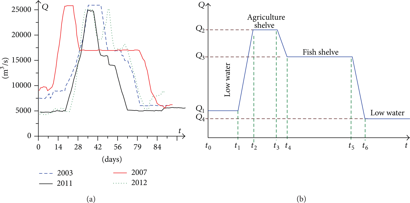
Examples of hydrographs for different years (a), structure of hydrograph and its main components (b).

A lot of different factors influence the hydrological regime of the flow, but the river bed roughness determines the most important properties of the water stream [5, 6]. Roughness coefficient n_M is an empirical parameter [7 –9]

n = n_{0} + n_{1} + n_{2} + n_{3} + n_{4} + n_{5} + n_{6},

(1)

accounting for inhibitory effects on the real bottom roughness in straight uniform channel (n₀), irregularities of the bottom (n₁) [10], variations in the geometry of the channel, meandered channel (n₂), various obstacles (n₃), vegetation (n₄) [11], turbulence (n₅) [12], and other additional hydrological resistances (n₆). In case of strong meandering, the parameter should be increased by about 30 percent. The value of roughness n_M in actual flood can vary quite widely in the range 0.01–0.2 [13 –15]. We are not able to calculate the effect of many factors n_i on the hydrological resistance. However, the parameterization of the roughness coefficient allows us to obtain reasonable results without detailed modeling of highly complex processes in the three-dimensional turbulent water flow [16, 17]. The problem with the roughness coefficient is very similar to the situation in the standard accretion disk model by Shakura and Sunyaev in which a key role is played by the so-called α-parameter determining the transfer rate of angular momentum in the gaseous disk around the compact object (black hole, neutron star, or white dwarf). The physical processes in accretion disks are highly dependent on the α-parameter [18], and the comparisons of model results with observational data enable us to estimate the value of α [19].

The main goal of our work is to estimate of the Volga River bed roughness coefficient for the modified Manning model based on the numerical simulations of the dynamics of shallow water. The information about the dynamics of water levels at the gauging stations η_obs^(m)(t) is used for direct comparison with the numerical results for the spring flood. For the northern part of Volga-Akhtuba Floodplain, we have long term data from three gauging stations (GSs) (http://gis.waterinfo.ru/): (1) GS “Volga Hydroelectric Station” (m = 1); (2) GS “Volgograd” near the river terminal (m = 2); and (3) GS “Svetlyj Jar” (m = 3) as shown in Figure 2. We make a quantitative comparison of η_mod^(m)(t) in the numerical model with observations on the hydrological stations η_obs^(m)(t). The model of shallow waters dynamics for northern part of VAF with the accounting of the real complex bed topography, bottom friction, the Coriolis force, infiltration and evaporation of water, and unstable working of the Volga Hydroelectric Station has been constructed. The numerical method integrating of the Saint-Venant equations is based on the combined method cSPH-TVD [20], which was specially designed to simulate flooding and drying over arbitraryirregular topography.

Figure 2:

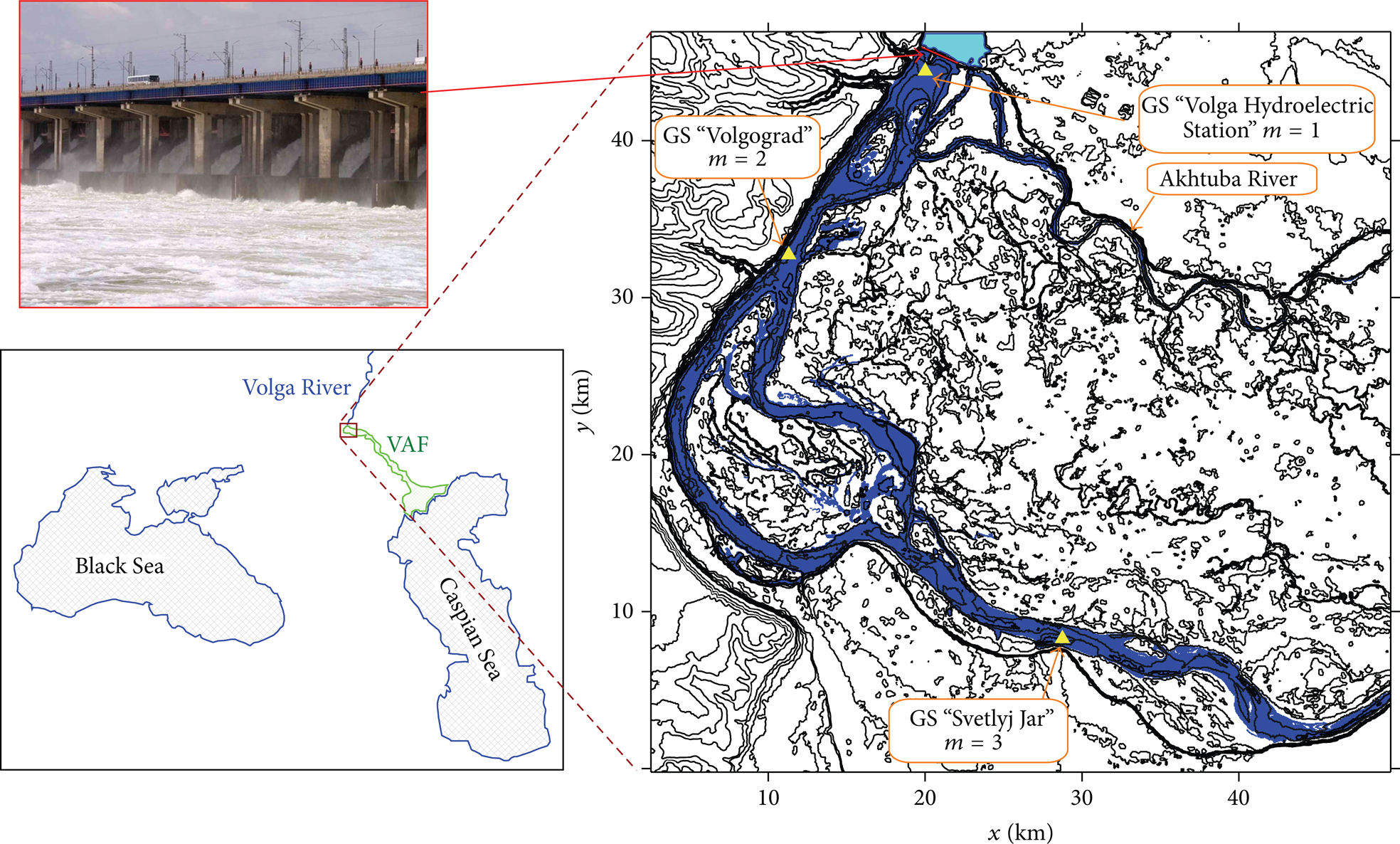
Topography of the Volga-Akhtuba Floodplain northern part and location of the gauging stations.

2. Mathematical Model

2.1. Basic Equations

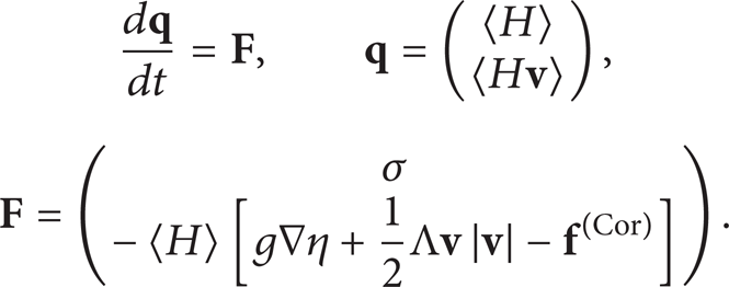
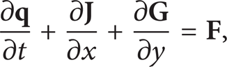
Numerical simulations were based on the Saint-Venant equations system accounting the horizontal forces [14, 21, 22]

\begin{matrix} \frac{\partial H}{\partial t} + \frac{\partial (H u)}{\partial x} + \frac{\partial (H v)}{\partial y} = σ, \\ \frac{\partial (H u)}{\partial t} + \frac{\partial}{\partial x} (H u^{2} + \frac{1}{2} g H^{2}) + \frac{\partial (H u v)}{\partial y} = - g H \frac{\partial b}{\partial x} + f_{x}^{(fric)} + f_{x}^{(Cor)} + f_{x}^{(visc)}, \\ \frac{\partial (H v)}{\partial t} + \frac{\partial (H u v)}{\partial x} + \frac{\partial}{\partial y} (H v^{2} + \frac{1}{2} g H^{2}) = - g H \frac{\partial b}{\partial y} + f_{y}^{(fric)} + f_{y}^{(Cor)} + f_{y}^{(visc)}, \end{matrix}

(2)

where u, v are components of the velocity vector v, H is the water depth, σ(x, y, t) = σ⁽⁺⁾ – σ⁽⁻⁾ is the sources function, g = 9.8 m/sec², f_x^(Cor) = 2HΩ_zv, and f_y^(Cor) = – 2HΩ_zu are the Coriolis force components f^(Cor), Ω_z is the vertical component of the angular speed of Earth's rotation on corresponding latitude, $f^{(fric)} = - (v / 2) Λ H \sqrt{u^{2} + v^{2}}$ is force of bottom friction, the value of hydraulic friction Λ = 2gn_M²/H^4/3 depends on the Manning roughness coefficient n_M [5], b(x, y) is the function of topography, and $f_{}^{(visc)} = (f_{x}^{(visc)}, f_{y}^{(visc)})$ is viscous force.

The level of the water free surface is equal η = H + b. Water losses from surface unit σ⁽⁻⁾ = σ^(e) + σ⁽ⁱⁿ⁾ are defined by evaporation σ^(e) and infiltration σ⁽ⁱⁿ⁾ rates. The value σ^(e) generally depends on the thermal and wind regimes and air humidity and convection. For VAF conditions during the flooding, it can be adopted σ^(e) = 2–5 millimeters per day. In our calculations, we have used the value σ⁽⁻⁾ = 3 centimeters per day.

The discharge Q(t) is calculated using the distribution of the water source σ⁽⁺⁾(x, y, t)

Q (t) = \iint_{S_{Q}}^{} σ^{(+)} (x, y, t) d x d y,

(3)

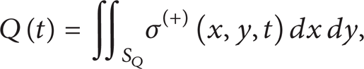
where S_Q is the area of the dam (see Figure 2), and we are neglecting the other sources.

Below, we consider only the case of f_x^(visc) = f_y^(visc) = 0. The quantitative impact of the viscous forces is discussed in Section 3.4.

2.2. Numerical Model

Numerical scheme of integrating equations (2) describing the complex of the nonsteady water flows over the irregular realistic terrain surface should satisfy the following conditions.

An important requirement is an adequate calculation of the dynamic boundaries between wet and dry beds [8, 15, 23]. The boundary “water-dry bottom” is essentially a nonstationary and simple traditional methods of regularization which provides a positivity of the numerical scheme [22]; however, it leads to large errors due to nonconservative procedures in methods.

Model needs both much subcritical flow (Froude number is $Fr = | v | / \sqrt{g H} ≪ 1$ in area almost still water) and supercritical regime (Fr > 1) without separating these zones.

The monotonicity property (absence of unphysical oscillations in the numerical solution) is quite a tough assignment in view of the irregular and/or discontinuous terrain b(x, y), containing a large number of sharp changes in the levels and kinks of the surface. A typical example is the surface of the ridge/ravine type, when the characteristic cross-scale of heterogeneity is comparable to the size of the numerical cell.

Further complicating factor is the requirement of stable calculating nonlinear structures like waterfall, vortex, shear flow, bore, expansion wave, and Tsunami.

The composed scheme of smoothed particle hydrodynamics—total variation diminishing (cSPH-TVD) algorithm is described in detail in the work [20] and satisfies the requirements above requirements. Here are the basic steps of the cSPH-TVD method to provide some additional important details which are necessary for understanding the finer points and sufficient for its implementation.

Let us construct the coordinate meshgrid (x_i = ih, y_j = jh, i = 0,1, …, N_x, j = 0,1, …, N_y) in Cartesian coordinate system. Then, we place the “fluid particle” with mass of $ρ 〈 H 〉 h^{2}$ , impulse of $ρ 〈 H v 〉 h^{2}$ , and mass center at the point $\tilde{r}$ at the center of each the grid cell. Mean value of quantities at Euler cells $〈 φ 〉 = (〈 H 〉, 〈 H v 〉)$ is related to integral characteristics of particles by formula $〈 φ 〉 = \int_{S (t)} φ d S / h^{2}$ , where S(t) is square of a fluid particle on the plane (x, y). The particle can move within the cell, but the position of the mass center of each particle ${\tilde{r}}_{i j}$ must coincide with the center of the cell r_ij = {x_i, y_j} at the beginning of each computational cycle at time t_n. All physical parameters A = {H, u, v} in (2) are defined nyz czby the values within the fixed cells A(x_i, y_j, t_n) ≡ A_{i, j}ⁿ and in the mass centers of the moving particles $\tilde{A} (x_{i}, y_{j}, t_{n}) \equiv {\tilde{A}}_{i, j}^{n}$ . We consider each of the steps ofthe cSPH-TVD-method.

(I) On Lagrange step, the exchanges of characteristics of fluid particles under the influence of sources/sinks, hydrodynamical and external forces are calculated using the approach of smooth particle hydrodynamics (SPH [24]). We rewrite the system of (2) in the conservative Lagrange form:

\begin{matrix} \frac{d q}{d t} = F, q = (\begin{pmatrix} 〈 H 〉 \\ 〈 H v 〉 \end{pmatrix}), \\ F = (\begin{pmatrix} σ \\ - 〈 H 〉 [g \nabla η + \frac{1}{2} Λ v | v | - f^{(Cor)}] \end{pmatrix}) . \end{matrix}

(4)

To approximate the spatial derivatives in (4), we use a modification of the SPH approach with the smoothing kernel $\hat{W}$ :

{(\nabla \tilde{η})}_{i, j} = \sum_{k = i - 1}^{i + 1} ‍ \sum_{ℓ = j - 1}^{j + 1} {〈 \tilde{η} 〉}_{k, ℓ} \nabla_{i, j} \hat{W} (\frac{| {\tilde{r}}_{i, j} - {\tilde{r}}_{k, ℓ} |}{h}) .

(5)

The kernel function corresponds to the Monaghan's cubic spline [25]

\hat{W} (ξ) = K_{w} {\begin{cases} 1 - \frac{3}{2} ξ^{2} + \frac{3}{4} ξ^{3}, & 0 \leq ξ \leq 1, \\ \frac{1}{4} {(2 - ξ)}^{3}, & 0 \leq ξ \leq 1, \\ 0, & ξ \geq 2, \end{cases}

(6)

where ξ = L/h and K_w is a constant determined by the normalization of $\hat{W}$ -kernel. In the classical approach, the SPH normalization condition for the planar case has the form [25]

\int_{0}^{\infty} ξ \hat{W} d ξ = 1, K_{w} = \frac{10}{7 π} .

(7)

But for the accurate approximation of the spatial derivatives in the expression (5) in the case of gently sloping profiles of the water level, we have used another normalization kernel:

\sum_{k = i - 1}^{i + 1} ‍ \sum_{ℓ = j - 1}^{j + 1} {〈 \tilde{η} 〉}_{k, ℓ} \frac{\partial \hat{W} (ξ)}{\partial ξ} \frac{ζ_{i, j}}{h L} = t g (β),

(8)

where β is the angle of the profile of the water level along the ζ-direction (ζ_{i, j} = x_i or ζ_{i, j} = y_j). Substituting (6) into (8), we have the normalization $K_{w} = (2 / 3) {[1 + \sqrt{2} {(2 - \sqrt{2})}^{2}]}^{- 1} ≃ 0.987 (10 / 7 π)$ . The numerical scheme is well balanced for such a renormalization, and we have good results as for modeling of the fluid level on a parabolic bottom and for the structure and dynamics of hydraulic jumps. Recurrence relations for each particle, which are based on an algorithm for time integration predictor-corrector, are as follows:

\begin{matrix} {\tilde{q}}_{i, j}^{n + 1 / 2} = q_{i, j}^{n} + \frac{Δ t_{n}}{2} F_{i, j} (q^{n}, r), {\tilde{r}}_{i, j}^{n + 1 / 2} = r_{i, j} + \frac{Δ t_{n}}{2} {\tilde{v}}_{i, j}^{n + 1 / 4}, \\ {\tilde{q}}_{i, j}^{n + 1} = q_{i, j}^{n} + Δ t_{n} F_{i, j} ({\tilde{q}}^{n + 1 / 2}, {\tilde{r}}^{n + 1 / 2}), \\ {\tilde{r}}_{i, j}^{n + 1} = r_{i, j} + Δ t_{n} {\tilde{v}}_{i, j}^{n + 1 / 2} . \end{matrix}

(9)

Stability of the numerical scheme in the first stage requires that each particle is not left out of the cell for the integration step Δt_n.

(II) At the second step (TVD), we calculate the mass and momentum fluxes due to the movement of fluid through the cell borders. This part of the algorithm is based on the system of the equations in conservative Euler form:

\frac{\partial q}{\partial t} + \frac{\partial J}{\partial x} + \frac{\partial G}{\partial y} = F,

(10)

where J = qu, G = qv are mass and momentum fluxes in the x- and y-directions, respectively. Finite-difference approximation of (10) has the form

q_{i, j}^{n + 1} = {\tilde{q}}_{i, j}^{n + 1} - \frac{Δ t_{n}}{h} (J_{i + 1 / 2, j}^{n + 1 / 2} - J_{i - 1 / 2, j}^{n + 1 / 2} + G_{i, j + 1 / 2}^{n + 1 / 2} - G_{i, j - 1 / 2}^{n + 1 / 2}),

(11)

where fluxes with half-integer indices $J_{i \pm 1 / 2, j}^{n + 1 / 2} = J ({\tilde{q}}_{i \pm 1, j}^{n + 1 / 2})$ and $G_{i, j \pm 1 / 2}^{n + 1 / 2} = G ({\tilde{q}}_{i, j \pm 1}^{n + 1 / 2})$ are calculated at the cell boundaries in time t_{n + 1/2} = t_n + Δt_n/2. We calculate the values using the corresponding solutions of the Riemann problem with the TVD-principle which provides that the total variation of the numerical solution does not increase in time [21, 26].

For solving the Riemann problem, we must calculate the values of conservative variables q on the left (L) and right (R) of the cell borders. This leads to a piecewise linear reconstruction of grid functions for the mass centers of the particles r_i^{n + 1/2}, which are located within the Euler cells (see Figure 3). The final condition for the stability of the cSPH-TVD numerical algorithm becomes

Δ t_{n} < \min_{i, j} (\frac{h}{2 | v_{i, j}^{n} |}, \frac{h}{| v_{i, j}^{n} | + \sqrt{g H_{i, j}^{n}}}) .

(12)

Figure 3:

Piecewise linear distribution of q for the scheme cSPH-TVD (a) and for schemes Godunov type (b). Here, x_i⁰ and x_i^{n + 1/2} are positions of the ith particle at time layers tⁿ and t^{n + 1/2}; λ ∈ [h/2; 3h/2] is the distance between the particles.

2.3. Digital Elevation Model (DEM)

Volga-Akhtuba Floodplain digital elevation model is based on the grids with a mesh size 20 and 50 meters. A brief description of the procedure for constructing DEM is as the following.

Remote sensing data is the basis of DEM. We use satellite data of ASTER GDEM 2 (Global DIGITAL Elevation Model) and SRTM X-SAR (Shuttle Radar Topography Mission) after additional processing of artifacts.

The coastlines of the hydrological system, based on the topographic data, are important components of the DEM.

We use the sailing directions to improve the model.

At the last stage, our GPS/GLONASS measurements allowed us to actualize the model of relief (see Figure 2).

2.4. The Computer Model

The calculations were performed on GPU using the parallel computing platform and the programming model CUDA. The calculating time of one spring flood of a duration of 100 days is equal to about 10 hours computer time on the Tesla C2070 processor, and the acceleration is about 216 compared to running on a single core of Intel Xeon 5320 CPU.

We have good results for standard tests [20] as follows.

The decay of an initial discontinuity of water depth and/or velocity [27, 28].

The dry-bed dam-break problem (Figure 4) [22, 28 –30].

The dynamics of surface gravity waves in the presence of nonuniform bottom topography [31, 32].

The research of process of long term propagation of the soliton for the study of the dispersion properties of the numerical scheme.

The formation of the hydraulic jump.

The calculation of steady and unsteady flows on a substantially nonuniform bottom relief, including discontinuous topography profiles [33, 34].

The Tsunami run-up to the sloping bank [35].

The sloshing motions in a vessel with parabolic bottom topography (Figure 5).

The flow with the waterfall (Figure 6).

The circular dam break over nonsmooth bed topography [21, 22, 36].

Figure 4:

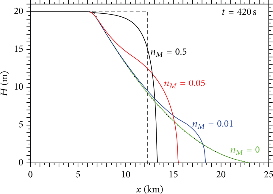
The dry-bed dam-break problem. The profiles of water depth at time t = 420 sec for different values of Manning n_M. The dotted line corresponds to the exact solution for n_M = 0; the dashed line is the initial profile.

Figure 5:

Moving boundary shallow water flow above parabolic bottom topography. The profiles of free surface level at two different times; the red circles are numerical solution for N = 100, and the solid lines are exact solution.

Figure 6:

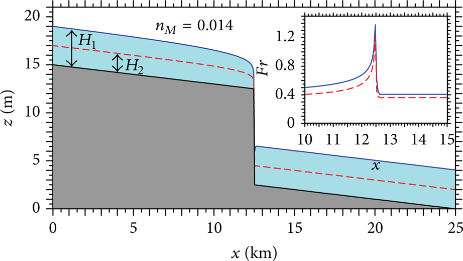
The flow with “waterfall.” Profiles of the free surface of the water level are shown. Solid blue line is H = 4 m, and the dashed red line is H = 2 m. The inset shows the distribution of the Froude number Fr near the discontinuity of topography.

3. Roughness Coefficient

3.1. Manning's Model

Roughness coefficient in the equation (see Section 1) is a complex phenomenological parameter, accounting for a large number of factors that we cannot estimate directly now. Manning's formula for the average velocity along the river bed [8, 37]

U = \frac{R_{g}^{2 / 3} s^{1 / 2}}{n_{M}}

(13)

depends on the bottom slope s and hydraulic radius R_g, averaged along the river. We have adopted R_g = H_av for a wide river (H_av is the average depth for the area along the river bed). This formula gives a reasonable estimation of hydrological parameters for the river Volga. For example, for the values R_g = H_av = 5 m, s = 5 · 10⁻⁵, and U = 1 m/sec, we obtain the roughness coefficient n_M ≃ 0.02 sec/m^1/3 (it is important to stress that the dimension is not indicated usually, and it is customary to write n_M ≃ 0.02).

3.2. Model of Constant Roughness Coefficient

Using the numerical simulations, we have studied how the roughness parameter determines the temporal dynamics of the water level at gauging stations η^(m)(t), m = 1,2, and 3 during spring flooding (see Figure 2). The results of the numerical simulations η_mod^(m)(t) have been compared with the observations at gauging stations η_obs^(m)(t) for the known function Q(t). In this section, we study the flood models with the constant roughness coefficient (n_M = const) throughout the numerical experiment.

Parameter n_M determines two values of the physical quantities, which can be compared with observations. This fact let us to estimate the value of roughness coefficient. First, the low-water model with a large value of the roughness coefficient provides a high level of the water by reducing the flow velocity according to the formula (12). Comparisons of the simulation results with the depth measurements H_obs^(m)(t) give us constraints on the value of the roughness coefficient. Second, during the spring water releases (see interval t₁-t₂ on hydrography in Figure 1), the rate of water level dη^(m)/dt is arising at gauging stations, and it highly depends on the value of n_M. The growth rate of the water level dη^(m)/dt increases in the case of large values of roughness, and, moreover, we have a high water level η^(m) [38]. Figure 7 shows this effect. The observed behavior of η_obs^(m)(t) during the spring water releases in the model with a constant coefficient of roughness cannot be explained in case n_M ≤ 0.06. A small hydraulic resistance with increasing of the water releases Q(t) leads to the formation of fast flow, and as a result, water level cannot rise up to observed values η_obs^(m)(t). In principle, the model with a constant roughness coefficient n_M ≃ 0.07 reproduces the observed growth Δη_obs^(m) ≃ 7 meters (see curve 1 in Figure 7 (b)). However, this requires an additional deepening of the river bed by 2 meters (see Figure 7 (c)). Thus, for the low-water period, the value of the roughness coefficient n_M = 0.02 will be used as the basic model.

Figure 7:

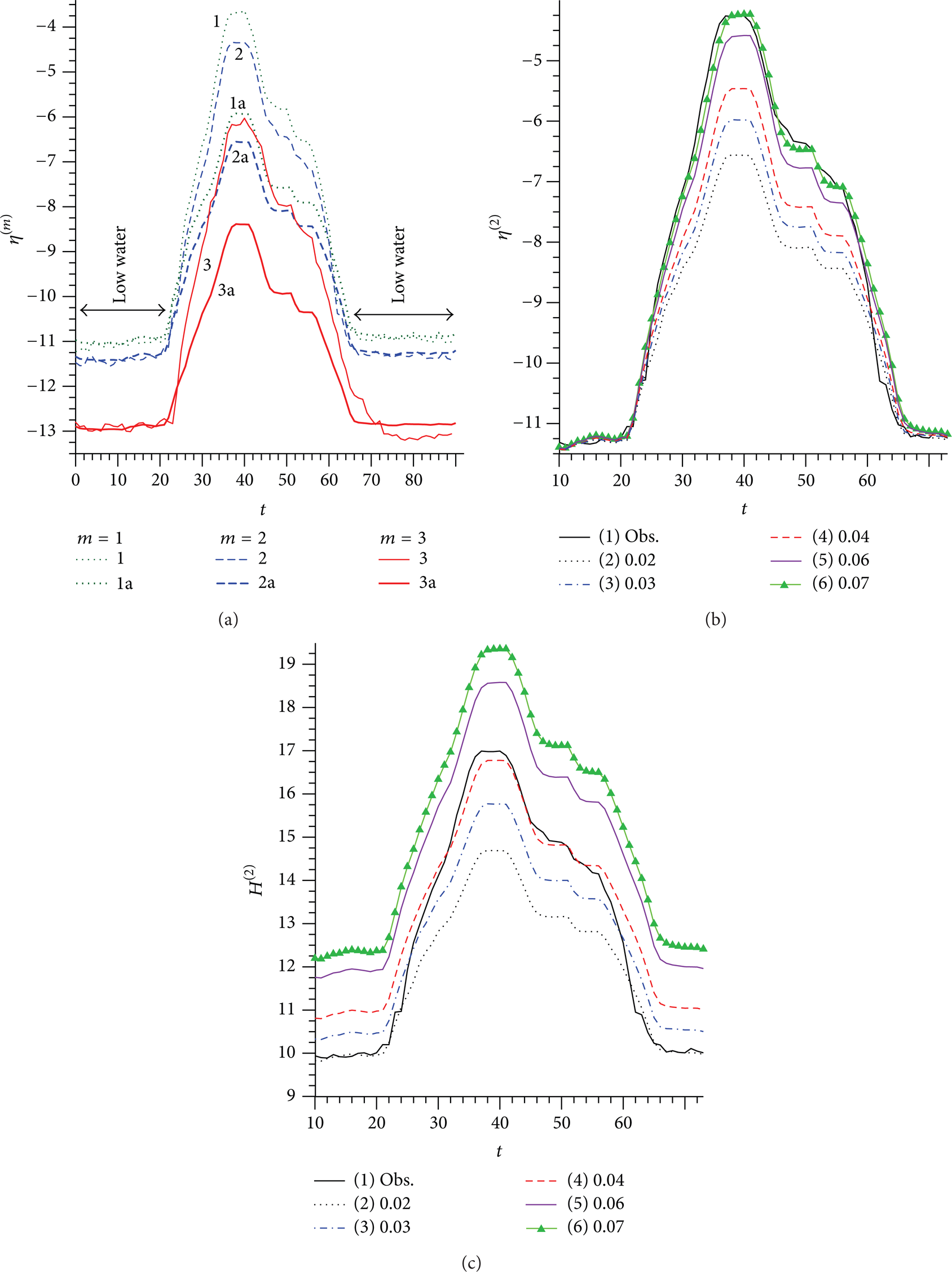
Water levels η^(m)(t) (meters) at gauging stations m = 1, 2, and 3 for different roughness values (time unit is a one day; t = 0 corresponds to 1 April 2011) (a) the data at gauging η_obs^(m)(t) (curves 1, 2, and 3) are compared with the model results η_mod^(m)(t) for n_M = 0.02 (curves 1a, 2a, and 3a); (b) the water levels at gauging “Volgograd” η_obs⁽²⁾(t) and η_mod⁽²⁾(t) for different values of the roughness coefficient n_M = 0.02, 0.03, 0.04, 0.06, and 0.07; (c) the comparison of water depths H⁽²⁾(t) for different values of Manning with the additional deepening of the Volga River bed in the model.

3.3. Parameterization of the Roughness Coefficient

The model with a constant n_M is not applicable during the flood, and we have the problem of creating a model for nonstationary roughness coefficient n_M(t). We restrict ourselves to the assumption that the roughness depends on the depth of the water in a river n_M(H). This parametrization allows to consider the increase flow resistance during the flood, and further the bottom structure is rebuilt, and the degree of turbulence increases. Let us restrict the simple model

n_{M} = n_{M}^{\min} + γ Δ H,

(14)

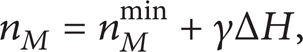
where ΔH(x, y, t) is the excess of depth comparing to the low-water state, when roughness is equal to n_M^min = 0.02. The directly proportional relationship n_M ∝ H_av is not contrary to statistics on the hydrological regime at a large sample of rivers [17]. Such a relation between n_M and H_av is more typical in the case of large rivers. We will fit the functions η_mod^(m)(t) to η_obs^(m)(t) to evaluate the coefficient γ which is determined by the maximum value of n_M^max.

Figure 8 shows the results of numerical experiments with different of n_M^max in the case (14). The maximum values of water levels for the observations and models agree with each other for n_M^max = 0.06–0.07. The model (14) with n_M^max ≃ 0.065 can increase the water level $η_{}^{(m)}$ by 7 meters. A model with a constant coefficient of roughness requires to explain the observations of larger values (n_M = 0.07), but in this case we cannot simulate the low-water state correctly. Note that a similar approach to the Yellow River has given Manning's coefficient n_M = 0.006–0.03 [14]. In the case of small rivers, the parameter n_M for the river Aa increase from winter value n_M = 0.04 to 0.15 and even 0.5 for summer situations with high amount of vegetation [5].

Figure 8:

A comparison of water levels from observations at three gauging stations with simulations in the model with time-dependent coefficient of roughness for different n_M^max: (1) η_obs^(m), (2) n_M^max = 0.07, (3) n_M^max = 0.065, (4) n_M^max = 0.06, and (5) n_M^max = 0.055.

It should be underlined that the model, with taking into account (14), is local and the coefficient n_M changes instantly in the case of variation in the water level. Obviously, the actual hydraulic resistance is characterized by the inertia. This is clearly seen in the decline stage of water in the so-called fish shelves (see F₁ and F₂ in Figure 8, and also the interval t₄-t₅ for hydrography in Figure 1) where there is a noticeable difference.

Increasing the water level in Volga by 5–7 meters is a necessary condition for the passage of the water into the territory between the Volga and Akhtuba (Figure 9). Otherwise, the water from the river Akhtuba cannot penetrate into the basic Floodplain through a network of narrow natural channels. Simulations with different values of water loss σ⁽⁻⁾ = 1, 2, 5, and 10 centimeters per day showed that this parameter affects weakly on the behavior of the levels at gauging stations within Volga river bed and only the character of flooding in the Floodplain varies greatly.

Figure 9:

Distributions of water in the flood plain in low water (a), in the time of maximum flooding (b), at the start of the fish shelve (c) (see Figure 1 (b)), and at the end of the fish shelve (d).

3.4. The Estimates of Viscous Forces

Let us discuss the influence of the turbulent viscosity on the dynamics of water in VAF. The components of the viscous force f_{x, y}^(visc) were used in the following form [39]:

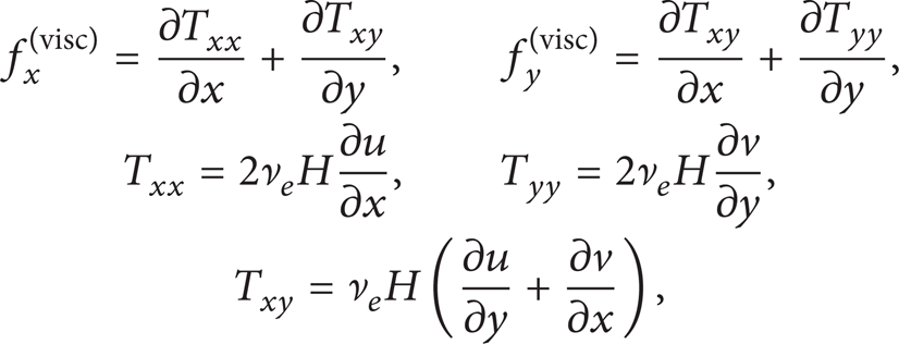
\begin{matrix} f_{x}^{(visc)} = \frac{\partial T_{x x}}{\partial x} + \frac{\partial T_{x y}}{\partial y}, f_{y}^{(visc)} = \frac{\partial T_{x y}}{\partial x} + \frac{\partial T_{y y}}{\partial y}, \\ T_{x x} = 2 ν_{e} H \frac{\partial u}{\partial x}, T_{y y} = 2 ν_{e} H \frac{\partial v}{\partial y}, \\ T_{x y} = ν_{e} H (\frac{\partial u}{\partial y} + \frac{\partial v}{\partial x}), \end{matrix}

(15)

where T_ij are the elements of the depth-averaged effective turbulent stress tensor in the vertical plane for the water layer,

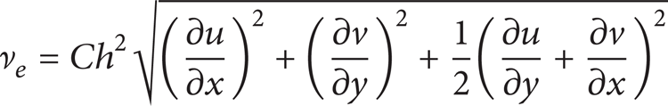
ν_{e} = C h^{2} \sqrt{{(\frac{\partial u}{\partial x})}^{2} + {(\frac{\partial v}{\partial y})}^{2} + \frac{1}{2} {(\frac{\partial u}{\partial y} + \frac{\partial v}{\partial x})}^{2}}

(16)

is the depth-averaged turbulent eddy viscosity, and C is close to the value of 0.04 [40].

The integral powers of the viscous force

A_{visc} = \int_{S_{H}}^{} | v \cdot f^{(visc)} | d S,

(17)

and the bottom friction force

A_{fric} = \int_{S_{H}}^{} | v \cdot f^{(fric)} | d S,

(18)

were calculated for typical conditions of VAF (S_H is flooded area). Figure 10 shows the relative contribution of viscous forces on the water dynamics. From numerical simulations, we obtain that the integral impact of the viscous forces is less than 2%. However, the viscous correction decreases additionally by about a factor of (50/20)² ≃ 6 if the cell size is reduced up to 20 meters. This result is a quite typical for the beds of the wide lowland rivers in contrast to the flows in lakes and seas where the role of the viscous forces can be more significant than the impact of the bottom friction forces [41, 42].

Figure 10:

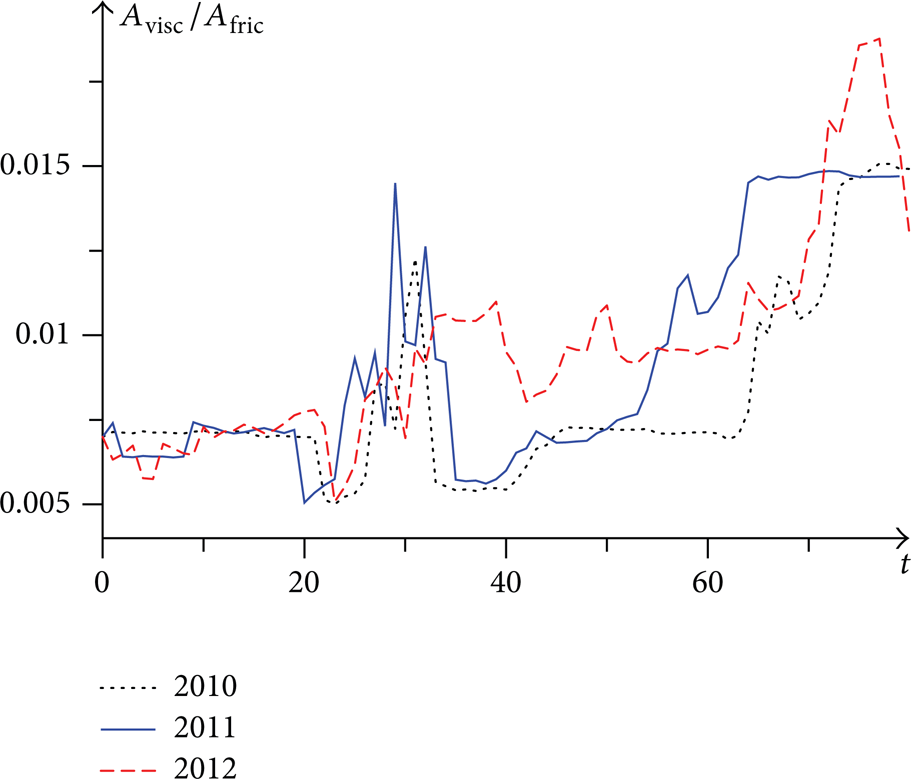
The relative power of viscous force versus time (days) for various years in the numerical experiments with h = 50 m.

4. Conclusions

We apply the shallow water model to the numerical simulation of spring flooding in Volga-Akhtuba Floodplain taking into account the real topography. Our results can be summarized as follows.

Models with a constant coefficient of roughness cannot reproduce the observed curves of the water levels at the three gauging stations in the northern part of the Volga-Akhtuba Floodplain in 2011. Parameterization of the roughness coefficient n_M(H) (see (14)) allows the agreeing of the results of hydrodynamic simulation with the hydrological observations. In the spring flooding in 2011 for low water, the roughness coefficient is 0.02, and at the stage of maximum water level, the value of n_M^max increases up to 0.06–0.07.

We plan to apply the model of the dynamics of shallow water for constructing an optimal hydrograph of water outflow through the dam during the spring period and control the hydrological regime in the Floodplain.

Footnotes

Acknowledgments

This work was supported by the Ministry of Education and Science of Russia (Project no. 8.2419.2011), Grants RFBR no. 13-01-97062, 13-07-97056. RFH no. 13-01-12015, and Federal Program “Scientific and Academic Specialists for Innovations in Russia, 2009–2013” (no. 14.B37.21.0284). Numerical simulations were implemented with supercomputer facilities “Lomonosov” and “Chebyshev” of the Moscow State University.

References

van de Wolfshaar

K. E.

Middelkoop

Addink

Winter

H. V.

, and Nagelkerke

L. A. J.

, “Linking flow regime, floodplain lake connectivity and fish catch in a large river-floodplain system, the Volga—akhtuba floodplain (Russian Federation),” Ecosystems, vol. 14, no. 6, pp. 920–934, 2011.

Górski

van den Bosch

L. V.

van de Wolfshaar

K. E.

, “Post-damming flow regime development in a large lowland river (Volga, Russian Federation): implications for floodplain inundation and fisheries,” River Research and Applications, vol. 28, no. 8, pp. 1121–1134, 2011.

Voronin

A. A.

Eliseeva

M. V.

Khrapov

S. S.

Pisarev

A. V.

, and Khoperskov

A. V.

, “The regimen control task in the eco-economic system “Volzhskaya hydroelectric power station—the Volga-Akhtuba floodplain” II. Synthesis of control system,” Control Sciences, no. 6, pp. 19–25, 2012.

Górski

Buijse

A. D.

Winter

H. V.

, “Geomorphology and flooding shape fish distribution in a large-scale temperate floodplain,” River Research and Applications, 2012.

De Doncker

Troch

Verhoeven

Bal

Meire

, and Quintelier

, “Determination of the Manning roughness coefficient influenced by vegetation in the river Aa and Biebrza river,” Environmental Fluid Mechanics, vol. 9, no. 5, pp. 549–567, 2009.

Y.-J.

and Chen

G.-X.

, “Non-uniform sediment transport model with the boundary-fitting orthogonal coordinate system,” Journal of Hydrodynamics, vol. 14, no. 1, pp. 64–68, 2002.

Cowan

W. L.

, “Estimating hydraulic roughness coefficients,” Agricultural Engineering, vol. 37, no. 7, pp. 473–475, 1956.

Bradford

S. F.

and Sanders

B. F.

, “Finite-volume model for shallow-water flooding of arbitrary topography,” Journal of Hydraulic Engineering, vol. 128, no. 3, pp. 289–298, 2002.

Coon

W. F.

, Estimates of Roughness Coefficients For Selected Natural Stream Channels With Vegetated Banks in New York, Ithaca, NY, USA, 1995.

10.

Omid

M. H.

Karbasi

, and Farhoudi

, “Effects of bed-load movement on flow resistance over bed forms,” Sadhana, vol. 35, no. 6, pp. 681–691, 2010.

11.

Tabacchi

Lambs

, and Guilloy

, “Impacts of riparian vegetation on hydrological processes,” Hydrological Processes, vol. 14, pp. 2959–2976, 2000.

12.

Stoesser

Wilson

C. A. M. E.

Bates

P. D.

, and Dittrich

, “Application of a 3D numerical model to a river with vegetated floodplains,” Journal of Hydroinformatics, vol. 5, no. 2, pp. 99–112, 2003.

13.

Arcement

G. J.

Jr. and Schneider

V. R.

, “Guide for selecting Manning's roughness coefficients for natural channels and food plains,” US Geological Survey Water-Supply Paper, vol. 2339, 1989.

14.

Xia

Lin

Falconera

R. A.

, and Wang

, “Modelling of man-made food routing in the lower Yellow River, Chi-na,” Water Management, vol. 165, pp. 377–391, 2012.

15.

Burguete

Garcia-Navarro

, and Aliod

, “Numerical simulation of runoff from extreme rainfall events in a mountain water catchment,” Natural Hazards and Earth System Sciences, vol. 2, pp. 109–117, 2002.

16.

Kitsios

Cordier

Bonnet

J.-P.

Ooi

, and Soria

, “Development of a nonlinear eddy-viscosity closure for the triple-decomposition stability analysis of a turbulent channel,” Journal of Fluid Mechanics, vol. 664, pp. 74–107, 2010.

17.

Baryshnikov

N. B.

, Hydraulic Resistance of River Beds, Izd. RGGU, Saint-Petersburg, Russia, 2003, (Russian).

18.

Khoperskov

A. V.

Khrapov

S. S.

, and Nedugova

E. A.

, “Dissipative-acoustic instability in accretion disks at a nonlinear stage,” Astronomy Letters, vol. 29, no. 4, pp. 246–257, 2003.

19.

Khoperskov

A. V.

and Khrapov

S. S.

, “Instability of high-frequency acoustic waves in accretion disks with turbulent viscosity,” Astronomy and Astrophysics, vol. 345, no. 1, pp. 307–314, 1999.

20.

Khrapov

S. S.

Khoperskov

A. V.

Kuz'min

N. M.

Pisarev

A. V.

, and Kobelev

I. A.

, “A Numerical scheme for sim-ulating the dynamics of surface water on the basis of the combined SPH-TVD approach,” Numerical Methods and Programming, vol. 12, pp. 282–297, 2011.

21.

Wang

J.-S.

and He

Y.-S.

, “Finite-volume TVD algorithm for dam-break flows in open channels,” Journal of Hydrodynamics, vol. 15, no. 3, pp. 28–34, 2003.

22.

Bollermann

Noelle

, and Lukáčová-Medvid'ová

, “Finite volume evolution galerkin methods for the shallow water equations with dry beds,” Communications in Computational Physics, vol. 10, no. 2, pp. 371–404, 2011.

23.

Toro

E. F.

, The Dry-Bed Problem in Shallow-Water Flows, College of Aeronautics report, 1990.

24.

Lee

and Han

, “Solving the Shallow Water equations using 2D SPH particles for interactive applications,” Visual Computer, vol. 26, pp. 865–872, 2010.

25.

Monaghan

J. J.

, “Smoothed particle hydrodynamics,” Annual Review of Astronomy and Astrophysics, vol. 30, no. 1, pp. 543–574, 1992.

26.

Lin

G.-F.

Lai

J.-S.

, and Guo

W.-D.

, “Finite-volume component-wise TVD schemes for 2D shallow water equations,” Advances in Water Resources, vol. 26, no. 8, pp. 861–873, 2003.

27.

Birman

and Falcovitz

, “Application of the GRP scheme to open channel flow equations,” Journal of Computational Physics, vol. 222, no. 1, pp. 131–154, 2007.

28.

Guo

Liu

R.-X.

Duan

Y.-L.

, and Li

, “A characteristic-based finite volume scheme for shallow water equations,” Journal of Hydrodynamics, vol. 21, no. 4, pp. 531–540, 2009.

29.

Mangeney

Heinrich

, and Roche

, “Analytical solution for testing debris avalanche numerical models,” Pure and Applied Geophysics, vol. 157, no. 6–8, pp. 1081–1096, 2000.

30.

Xia

Lin

Falconer

R. A.

, and Wang

, “Modelling dam-break flows over mobile beds using a 2D coupled approach,” Advances in Water Resources, vol. 33, no. 2, pp. 171–183, 2010.

31.

, “A well-balanced gas-kinetic scheme for the shallow-water equations with source terms,” Journal of Computational Physics, vol. 178, no. 2, pp. 533–562, 2002.

32.

Bulatov

O. V.

and Elizarova

T. G.

, “Regularized shallow water equations and an efficient method for numerical simulation of shallow water flows,” Computational Mathematics and Mathematical Physics, vol. 51, no. 1, pp. 160–173, 2011.

33.

Yang

Yin

Zhong

, and Dong

, “Rossby solitary waves generated by wavy bottom in stratified fluids,” Advances in Mechanical Engineering, vol. 2013, Article ID 289269, 10 pages, 2013.

34.

Ozmen-Cagatay

and Kocaman

, “Dam-break flow in the presence of obstacle: experiment and CFD simulation,” Engineering Applications of Computational Fluid Mechanics, vol. 5, no. 4, pp. 541–552, 2011.

35.

Adityawan

M. B.

and Tanaka

, “Bed stress assessment under solitary wave run-up,” Earth Planets and Space, vol. 64, pp. 945–954, 2012.

36.

Bohr

Dimon

, and Putkaradze

, “Shallow-water approach to the circular hydraulic jump,” Journal of Fluid Mechanics, vol. 254, pp. 635–648, 1993.

37.

Chow

V. T.

, Open-Channel Hydraulics, McGraw-Hill Book Company, New York, NY, USA, 1959.

38.

Pisarev

A. V.

Khrapov

S. S.

Agafonnikova

E. O.

, and Khoperskov

A. V.

, “Numerical model of shallow water dynamics in the channel of Volga: estimation of roughness,” Bulletin of Udmurt University. Mathematics, Mechanics, Computer Science, no. 1, pp. 114–130, 2013, http://vst.ics.org.ru/journal/article/1981/.

39.

Krámer

and Józsa

, “Solution-adaptivity in modelling complex shallow flows,” Computers and Fluids, vol. 36, no. 3, pp. 562–577, 2007.

40.

Wang

, “Importance of subgrid-scale parameterization in numerical simulations of lake circulation,” Advances in Water Resources, vol. 26, no. 3, pp. 277–294, 2003.

41.

Szydlowski

and Twarog

, “Numerical investigation of flooding of real-topography developed areas following river embankment failure,” TASK Quarterly, vol. 10, no. 3, pp. 321–338, 2006.

42.

Chang

T.-J.

Kao

H.-M.

Chang

K.-H.

, and Hsu

M.-H.

, “Numerical simulation of shallow-water dam break flows in open channels using smoothed particle hydrodynamics,” Journal of Hydrology, vol. 408, no. 1–2, pp. 78–90, 2011.

The Numerical Simulation of Shallow Water: Estimation of the Roughness Coefficient on the Flood Stage

Abstract

1. Introduction

2. Mathematical Model

2.1. Basic Equations

2.2. Numerical Model

2.3. Digital Elevation Model (DEM)

2.4. The Computer Model

3. Roughness Coefficient

3.1. Manning's Model

3.2. Model of Constant Roughness Coefficient

3.3. Parameterization of the Roughness Coefficient

3.4. The Estimates of Viscous Forces

4. Conclusions

Footnotes

Acknowledgments

References