A Low-Cost Anchor Placement Strategy for Range-Free Localization Problems in Wireless Sensor Networks

Abstract

The deployment of anchor nodes (or beacon nodes) is a key element in the design of range-free localization schemes for wireless sensor networks (WSNs). The majority of range-free localization schemes deploy numerous anchor nodes within the monitored region. However, in certain cases (e.g., hazardous areas), it may not be possible to manually install anchor nodes within the monitored region of a WSN. In this study, very few anchor nodes are installed at the boundary of a WSN monitored region to estimate the locations of unknown sensors. The locations of the unknown sensors are estimated based on the minimum hop counts to the anchor nodes. The average hop distance is estimated by applying parameters derived from prior experiments. The simulation results show that the range error of the proposed localization scheme can be as low as 0.15. The localization accuracy, computation cost, and communication cost of the proposed scheme are compared with those of the well-known DV-Hop method.

1. Introduction

Wireless sensor networks (WSNs) have recently received unprecedented attention due to their potential wide-ranging applications such as military surveillance, healthcare, home automation, tracking, and habitat monitoring. A WSN consists of a large number of small and inexpensive smart sensors working collaboratively to achieve a common objective and one or more sinks (or base stations) collecting data from all sensor devices. Sensors are being deployed to monitor or disseminate information of various environmental or physical conditions, such as sound, temperature, motion, pressure, pollutants, and vibration.

The energy consumed for transmitting a wireless radio signal is in proportion to the square of the distance, or even a higher order if the environment contains hindrances. Thus, in a WSN, multihop routing is usually considered as an alternative to direct communication for transmitting data to the sink. The majority of WSN routing algorithms count on knowledge of the precise location of each sensor. However, for specific hazardous environments, it is hard to measure the positions of sensors manually. Fortunately, various localization techniques can be used to estimate the locations of sensors. Perhaps the most popular localization approach is to install the GPS on the sensors in a WSN. Despite the declining cost of GPS receivers, they remain too cost- and energy-inefficient for installing in a WSN. Therefore, other techniques need to be developed for localization problems in WSNs.

There are two general classes of WSN localization technology: (1) range-based approaches and (2) range-free approaches [1]. Range-based approaches require sensor nodes to be positioned using additional devices, such as directional antennas, ultrasonic detectors, antenna arrays, and signal-strength receivers. By contrast, range-free approaches do not rely on any extra hardware for additional information. Rather, they depend solely on the basic properties of sensor nodes, the network connectivity, and the information of their direct neighbors.

An established range-free localization method called the DV-Hop method was proposed by Niculescu and Nath in [2]. The DV-Hop method is based on classical distance vector exchange from general packet-switched network protocols. In DV-Hop, anchor nodes flood their positions to all nodes in the network. Each node computes the minimum distance in hops to every anchor node. Anchor nodes compute an average distance per hop (i.e., hop size) to other anchors. The hop size of each anchor is then flooded to the whole network to facilitate unknown sensors to compute their positions. Each unknown sensor estimates the distances to their respective neighboring anchors based on the number of hop counts and the hop size of the anchor with the smallest hop count. The unknown sensors subsequently multilaterate their positions based on the estimated distances to their nearest neighboring anchors.

Different from the DV-Hop, the MDS-MAP [3] method uses the hop count to construct a proximity matrix as a relative map by the multidimensional scaling technology, and it then obtains absolute locations by some linear transformation. There are three major steps in the MDS-MAP. The first step is to form the distance matrix with distances between all pairs of nodes in the network. In the absence of anchors, the distance is obtained by multiplying the hop count with the radio range. In the second step, singular vector decomposition (SVD) is performed to get an initial relative map of the nodes in the monitored region. The last step performs some linear transformations according to the distances between anchors whenever applicable. Otherwise, the relative map would be the result of SVD. The time complexities of the first two steps are $O(n^3)$ , where n is the number of nodes in the network, while the complexity of the last step depends on the network topology.

APIT [4] employs an area-based approach to perform location estimation by dividing the monitored area into triangular regions between anchor nodes. Each unknown node runs the point-in-triangle (PIT) tests to find the triangle regions it resides in. However, it is hard for the unknown nodes to perform the exact PIT test. The authors presented an approximate PIT test, in which the node is only required to be able to determine whether any one of its neighbors is farther or closer to all of the three anchors that form its residing triangle. For better localization accuracy, the suggested degree of connectivity should be greater than six, and, in order to improve accuracy, APIT assumes that the anchors have radio ranges that are 10 times larger than those of ordinary nodes.

Localization refers to the ability of determining the position (absolute or relative) of an unknown sensor node, with an acceptable accuracy. The estimation accuracy of unknown sensors is usually affected by the location of anchor nodes. Numerous studies have examined the influence of anchor positions on the estimation accuracy of unknown sensor nodes [5–8]. In [7], the authors sought to identify anchor locations that would obtain the highest accuracy for all target sensor node positions. They selected anchors that offered the minimum of the mean Cramér-Rao bound (CRB). They studied the optimal anchor positions for three to eight anchors in the following two noise models: (1) the additive noise model (aNm) and (2) the multiplicative noise model (mNm). The authors concluded that the CRB achieved the lowest mean when the anchors were located equidistantly at the boundary of a square region for four and eight anchor nodes.

In [8], the authors installed four anchors in an 8 × 8 square region to estimate the location of unknown sensors by using a multihop setup, where neighboring nodes with unknown positions assisted other nodes to estimate their locations by acting as anchor points. They concluded that the anchor nodes should be installed at the perimeter of the network so that their proposed localization algorithms can have minimal variance of the mean error bounds.

This study proposes a low-cost and an effective localization scheme for WSNs. The scheme requires fewer than 16 anchor nodes placed at the boundary of a monitored region. The location of each unknown sensor is estimated using bilateration (employing two anchors) or multilateration (employing more than two anchors). For multilateration, we equidistantly installed the anchors at the boundary of the monitored square region. The distances between unknown sensors and anchor nodes are estimated based on their minimum hop counts, instead of applying noise models.

This study shows that additional anchor nodes increase the accuracy of location estimation. However, the accuracy ratio converges when the number of anchor nodes reaches a certain threshold. This study also provides a performance comparison, including communication cost and computation cost, between the proposed scheme and the DV-Hop method to demonstrate the superiority of the proposed scheme.

The remainder of this paper is organized as follows. Section 2 introduces a mechanism for estimating the distance of each unknown node to the anchor nodes, and Section 3 details the proposed localization scheme. Section 4 proposes two anchor placement strategies and compares their performance. Section 5 provides simulations of the proposed localization scheme and a comparison of its performance with the DV-Hop method and some renowned schemes. Lastly, Section 6 offers a conclusion.

2. Distance Estimation of Unknown Sensors

In the proposed localization scheme, few (i.e., 2–16) anchor nodes are installed at the boundary of a monitored square region to estimate the positions of unknown sensors. Two major stages are conducted to locate the unknown sensors.

Preliminary Stage

• (1)

Obtain the minimum hop counts from the unknown sensors to each anchor node.

(2)

Estimate the distances between the unknown sensors and the anchor nodes based on their corresponding minimum hop counts.

Localization Stage. Apply bilateration (i.e., for two anchors) or multilateration (i.e., for 4–16 anchors) to estimate the position of the unknown sensors.

This study assumes that (1) the network is connective (the theoretical expected number of local neighbor nodes to ensure connectedness is between 2.195 and 10.526, and simulation experiments suggest at least 5 [9]), (2) sensors are uniformly distributed in the monitored region, and (3) all sensors are homogeneous.

We extend the distance estimation method proposed in [10] from two anchor nodes to k ( $2\leqq k\leqq 16$ ) anchor nodes for the preliminary stage. For the sake of the self-containment of the paper, the procedures of how to obtain the minimum hop counts for the unknown sensors and how to estimate the hop distance between unknown sensors and anchor nodes are briefly described in the next two subsections. For more details, please refer to [10]. The localization stage is discussed in Section 3.

2.1. Obtain the Minimum Hop Counts from the Unknown Sensors to Each Anchor Node

Suppose that there are k anchor nodes, where k ranges from 2 to 16 (the influence of the number of anchor nodes is discussed in Section 4), and each anchor node is initially allowed to broadcast a Hello packet to its neighbor nodes. The Hello packet consists of the following two fields: (1) Min_hc (minimum hop count to the source node), which is initialized at zero, and (2) the source anchor node ID.

Each sensor stores a k-tuple vector ( ${\text{hop}}_{\mathrm{1}},{\text{hop}}_{\mathrm{2}},\dots ,{\text{hop}}_k$ ), where ${\text{hop}}_i$ is the current minimum hop count to Anchor Node i, $1\le i\le k$ . Each entry of the vector is initially set at positive infinity. Once a sensor has received a Hello packet from Anchor Node i, where $1\le i\le k$ , it examines the Min_hc value of the packet. If ${\text{hop}}_i$ of the sensor is greater than (Min_hc + 1), the sensor increases Min_hc by one before the Hello packet is forwarded to its neighbor nodes and accordingly updates ${\text{hop}}_i$ to the new Min_hc value. Otherwise, the current incoming Hello packet is discarded.

After completing this procedure, each unknown sensor obtains the minimum hop-count value to each anchor node. The values in each unknown sensor are denoted as a k-tuple ( ${\text{hop}}_{\mathrm{1}},{\text{hop}}_{\mathrm{2}},\dots ,{\text{hop}}_k$ ), where ${\text{hop}}_i$ is the minimum hop count to Anchor Node i, $1\le i\le k$ .

2.2. Estimate the Hop Distances between Unknown Sensors and Anchor Nodes

Let n be the total number of sensors, let CR be the communication range of each sensor, and let w be the length of the monitored square region. The probability that sensor v is within the communication range of sensor u is $\pi \times \text{C}{\text{R}}^2/w^2$ . Because the total number of sensors is n, the expected number of neighbor nodes $(\rho )$ for u is $(n-\mathrm{1})(\pi \times \text{C}{\text{R}}^2/w^2)$ . For example, if $n=300$ , $\text{CR}=30$ , and $w=200$ , then $\rho =(\mathrm{300}-\mathrm{1})\times (3.14\times {30}^2/{200}^2)\cong 21$ . A previous study [11] gave a more precise calculation of the node degree which takes the border effect into consideration. According to [8], $\rho =(n-\mathrm{1})(\pi r^2-8/3r^3+(11/3-\pi )r^4)$ , where $r=\text{CR}/w$ . Therefore, $\rho \cong \mathrm{19}$ for this case.

According to [12], the probability of a message flooding along the straight-line path between nodes is ≥0.85 if the number of expected neighboring nodes is ≥15. Therefore, in the same example, if $\text{CR}=20$ , then $\rho >15$ if $n>478$ . Alternatively, if $\text{CR}=30$ , then $\rho >15$ if $n>213$ . Two extreme cases of the messages being forwarded along the straight-line paths are presented in the following.

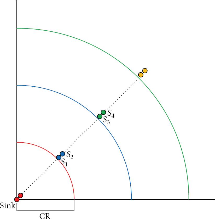
The average hop distance between sensors is determined by the node density and the communication range of the sensors in the monitored region [10–12]. When the node density is high, each sensor may have a larger number of neighbor nodes. Therefore, it is very likely that some sensor nodes are located at the edge of each one-hop broadcast boundary of an anchor node. As shown in Figure 1, in this extreme case, there always exist sensor nodes at the edge of the one-hop broadcast boundary of the sink. Therefore, under this circumstance, the maximum distance of an unknown sensor to the sink with minimum hop count m is $m\times \text{CR}$ .

Figure 1

An extreme case of sensors (red nodes) routing with minimum hop count to the sink along straight-line paths (the dotted lines).

Observation 1.

Let CR be the communication range. If messages are forwarded along straight-line paths, the maximum distance of an unknown sensor with minimum hop count m from the sink is $m\times \text{CR}$ .

The other extreme case happens when the node density is low and each node has a small number of neighbors, yet the network remains connective. As shown in Figure 2, sensors are pairs located proximally to the edge of the one-hop broadcast boundary of the sink. The first node in each pair is within the scope of the second node of the preceding pair, but it is immediately outside the scope of the first node of the preceding pair. At the same time, the second node in each pair is immediately outside the scope of the second node of the preceding pair.

For example, in Figure 2, $S_3$ is within the communication range of $S_2$ , but it is immediately outside the scope of $S_1$ . $S_4$ is immediately outside of the scope of $S_2$ . Thus, the minimum distance of sensors with hop count m routing along a straight-line path is $\lfloor m/2\rfloor \times \text{CR}+ϵ$ , where ϵ is summation of the distances of each node pair in the path. For example, the hop count of $S_3$ is 4, and the distance to the sink is $\mathrm{2}\times \text{CR}+ϵ$ . The hop count of $S_4$ is 5, and the distance is $\mathrm{2}\times \text{CR}+{ϵ}^{\prime }$ , where ${ϵ}^{\prime }>ϵ$ . If the two nodes in each pair are very close to each other and still comply with the conditions, the small value ϵ can be ignored and the minimum distance of sensors routing along a straight-line path with hop count m is $\lfloor m/2\rfloor \times \text{CR}$ .

Figure 2

The case of minimum distance to the sink when the forwarding of messages is along a straight line, in which sensors are pairs located proximally to the edges of the one-hop broadcast boundaries of the sink.

Observation 2.

Let CR be the communication range. If messages are forwarded along straight-line paths, the minimum distance of a sensor with hop count m from the sink is $\lfloor m/\mathrm{2}\rfloor \times \text{CR}$ .

From Observations 1 and 2, we conclude that if packets are forwarded along a straight-line path, the distance from any sensor with minimum hop count m to the sink is between $\lfloor m/2\rfloor \times \text{CR}$ and $m\times \text{CR}$ (ϵ is ignored). Therefore, if an unknown sensor S is with minimum hop counts ( ${\text{hop}}_{\mathrm{1}},{\text{hop}}_{\mathrm{2}},\dots ,{\text{hop}}_k$ ) to each anchor node, then the following formula can be applied to approximate the distances (i.e., $d_1,d_2,\dots ,d_k$ ) from sensor S to Anchor Node 1, Anchor Node 2 $,\dots$ , Anchor Node k, respectively. Consider

$$\begin{array}{cc}& d_i=\left\{\lfloor \frac{{\text{hop}}_i}{\mathrm{2}}\rfloor +\left[\left({\text{hop}}_i-\lfloor \frac{{\text{hop}}_i}{\mathrm{2}}\rfloor \right)\times {\alpha }_i\right]\right\}\times \text{CR},\end{array}$$

(1)

where $i=1,\dots ,k$ and ${\alpha }_i$ is a parameter between 0 and 1. To simplify the calculation, this study applied an identical α value for each ${\alpha }_i$ under the same deployment condition. The determination of α is discussed in Section 4.

3. The Localization Scheme

In this study, 2–16 anchor nodes were used to estimate the positions of unknown sensors. For the WSNs that require coarse-grained localization, the bilateration localization method (BLM) is applied. The BLM, which was introduced by Chen et al. in [10], uses only two anchor nodes and employs a basic geometry property—the intersection of two circles—to estimate the position of an unknown sensor. For the WSNs that require fine-grained localization, the least-squares multilateration localization method (LSMLM) with 4 to 16 anchor nodes is applied based on the Newton-Raphson method.

3.1. Bilateration Localization Method

In the BLM, only two anchor nodes are used to estimate the location of unknown sensors. The two anchor nodes are installed at the lower-left (Sink X) and lower-right (Sink Y) corners of a monitored square region (Figure 3).

Figure 3

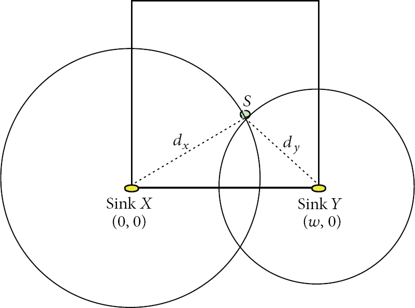
Two sinks are located at the lower-left corner and the lower-right corner, respectively, of the monitored region.

Suppose that Sink X is installed at (0,0) and Sink Y is installed at $(w,0)$ , where w is the length of the monitored square region. Given an unknown sensor S with coordinate $(x,y)$ , let the distances from S to Sink X and Sink Y be $d_x$ and $d_y$ , respectively. Values of x and y can be calculated from the following equations derived from the intersection of two circles with radii $d_x$ and $d_y$ centered at (0,0) and $(w,0)$ :

$$\begin{array}{l}{\left(x-\mathrm{0}\right)}^{\mathrm{2}}+{\left(y-\mathrm{0}\right)}^{\mathrm{2}}={d_x}^{\mathrm{2}},\\ {\left(x-w\right)}^{\mathrm{2}}+{\left(y-\mathrm{0}\right)}^{\mathrm{2}}={d_y}^{\mathrm{2}}.\end{array}$$

(2)

Thus, $x=({d_x}^{\mathrm{2}}-{d_y}^{\mathrm{2}}+w^{\mathrm{2}})/\mathrm{2}w$ , and $y=\pm \sqrt{{d_x}^{\mathrm{2}}-x^{\mathrm{2}}}$ .

Because the unknown sensor S is located in the first quadrant of the Cartesian coordinate system, only the positive solution of y can be taken. Therefore, the coordinate of sensor S is

$$\begin{array}{cc}& \left(\frac{{d_x}^{\mathrm{2}}-{d_y}^{\mathrm{2}}+w^{\mathrm{2}}}{\mathrm{2}w},\sqrt{{d_x}^{\mathrm{2}}-{\left(\frac{{d_x}^{\mathrm{2}}-{d_y}^{\mathrm{2}}+w^{\mathrm{2}}}{\mathrm{2}w}\right)}^{\mathrm{2}}}\right).\end{array}$$

(3)

Note that, in order to obtain a real solution using (2), the following inequality should be stratified:

$$\begin{array}{cc}& d_x+d_y\ge w.\end{array}$$

(4)

This constraint will be considered when estimating $d_x$ and $d_y$ in (1).

3.2. Least-Squares Multilateration Localization Method

Although the BLM is appealing because the number of required anchor nodes is very small, the range error (defined in Section 4) of localization is slightly high. To reduce the error rate of localization, in this study, additional anchor nodes (from 4 to 16) were added to the localization scheme. The LSMLM is used to estimate the locations of the unknown nodes. In the following subsections, the mathematical background of the LSMLM is detailed, and a common least-squares solver is offered.

3.2.1. Multilateration of Newton-Raphson/Least Squares

Given k nodes with known Cartesian positions $b_i$ , $i=1,\dots ,k$ , and potentially noisy range measurements $r_i$ from the known nodes to an unknown node s, the multilateration problem is to identify the most probable position of s. Multilateration is typically conducted by minimizing the squared error between the predicted distance $\parallel s_{}-b_i\parallel$ and the observed ranges $r_i$ . Consider

$$\begin{array}{cc}& s=\underset{s}{\text{argmin}\hspace{0.17em}}E\left(s\right),\end{array}$$

(5)

$$\begin{array}{ll}& E\left(s\right)=\sum _{i=1}^k{\left(\parallel s-b_i\parallel -r_i\right)}^2.\end{array}$$

(3′)

Expression (5) can be solved using Newton-Raphson/least squares, described in [13], as follows. First, approximate the error function $e(s,b_i)=\parallel s-b_i\parallel -r_i$ in ( 3 ′ ) with a first-order Taylor series regarding $s_0$ :

$$\begin{array}{l}e\left(s,b_i\right)\approx e\left(s_{\mathrm{0}},b_i\right)+\nabla e\left(s_{\mathrm{0}},b_i\right)\left(s-s_{\mathrm{0}}\right)\\ \hspace{1em}\hspace{1em}\hspace{1em}=\nabla e\left(s_0,b_i\right)s-\left(-e\left(s_0,b_i\right)+\nabla e\left(s_0,b_i\right)s_0\right),\end{array}$$

(6)

where $\nabla e(s_{\mathrm{0}},b_i)$ is the gradient of $e(s,b_i)$ at $s_{\mathrm{0}}$ , and the value is $(s_{\mathrm{0}}-b_i)/\parallel s_{\mathrm{0}}-b_i\parallel$ .

Next, substitute this approximation into (5):

$$\begin{array}{cc}& s\approx \underset{s}{\text{argmin}\hspace{0.17em}}\sum _{i=\mathrm{1}}^k{\left(\nabla e\left(s_{\mathrm{0}},b_i\right)s-\left(-e\left(s_{\mathrm{0}},b_i\right)+\nabla e\left(s_{\mathrm{0}},b_i\right)s_{\mathrm{0}}\right)\right)}^{\mathrm{2}}.\end{array}$$

(7)

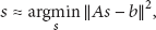
Stacking the terms yields

$$\begin{array}{cc}& s\approx \underset{s}{\text{argmin}\hspace{0.17em}}{\parallel As-b\parallel }^{\mathrm{2}},\end{array}$$

(8)

where

$$\begin{array}{cc}& A=\left[\begin{array}{c}\nabla e\left(s_{\mathrm{0}},b_{\mathrm{1}}\right)\\ \nabla e\left(s_{\mathrm{0}},b_{\mathrm{2}}\right)\\ ⋮\\ \nabla e\left(s_{\mathrm{0}},b_k\right)\end{array}\right],\end{array}$$

(9)

$$\begin{array}{cc}& b=\left[\begin{array}{c}\left(-e\left(s_0,b_1\right)+\nabla e\left(s_0,b_1\right)s_0\right)\\ \left(-e\left(s_0,b_2\right)+\nabla e\left(s_0,b_2\right)s_0\right)\\ ⋮\\ \left(-e\left(s_0,b_k\right)+\nabla e\left(s_0,b_k\right)s_0\right)\end{array}\right].\end{array}$$

(10)

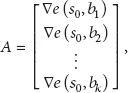
The right side of (8) is suitable for being solved using an off-the-shelf least-squares solver. If $b_i$ and $r_i$ are accurate, the resulting s will be a good estimated position for the unknown sensor.

The multilateration method is summarized as follows.

Step 1.

Estimate the distance $r_i$ between the unknown node and Anchor Node i, where $i=\mathrm{1,2},\dots ,k$ (the estimation process of the distances $r_i$ was described in Section 2).

Step 2.

Select $s_{\mathrm{0}}$ as a starting point for minimization. This selection is arbitrary, although the centroid $\stackrel{-}{b}$ is suitable:

$$\begin{array}{cc}& \stackrel{-}{b}=\frac{\mathrm{1}}{k}\sum _{i=\mathrm{1}}^k{b}_i.\end{array}$$

(11)

Step 3.

Compute A and b by using $s_{\mathrm{0}}$ to (9) and (10).

Step 4.

Compute $s_{\mathrm{0}}^{\prime }={\text{argmin}}_x\hspace{0.17em}{\parallel Ax-b\parallel }^{\mathrm{2}}$ by using a least-squares solver.

Step 5.

If $|E(s_{\mathrm{0}})-E(s_{\mathrm{0}}^{\prime })|<ϵ$ , then $s_{\mathrm{0}}^{\prime }$ is the solution; otherwise, set $s_{\mathrm{0}}=s_{\mathrm{0}}^{\prime }$ , and go to Step 3.

3.2.2. Least-Squares Solver

To solve the minimization problem of Step 4 in the previous multilateration method, an expression for the square of the Euclidean norm on $R^2$ can be applied [14]. For any vector v, the square of the Euclidean norm can be expressed as ${\parallel v\parallel }_{}^2=v^{T}v$ . Hence,

$$\begin{array}{l}{\parallel Ax-b\parallel }_{}^{\mathrm{2}}={\left(Ax-b\right)}^T\left(Ax-b\right)\\ \hspace{1em}\hspace{1em}\hspace{1em}\hspace{0.17em}\hspace{0.17em}=x^T{A}^{T}Ax-\mathrm{2}{x}^T{A}^{T}b+b^{T}b.\end{array}$$

(12)

Regarding (12) as a function of x, to minimize this expression, we need to set its gradient to zero:

$$\begin{array}{l}\mathrm{2}{A}^{T}Ax-\mathrm{2}{A}^{T}b=\mathrm{0}.\mathrm{\hspace{0.17em}\hspace{0.17em}}\\ \text{Thus},\hspace{0.17em}\hspace{0.17em}{A}^{T}Ax=A^{T}b.\end{array}$$

(13)

Equation (13) is called the normal equation for the linear least-squares problem. This equation has a unique solution provided that all of the columns of matrix A are linearly independent. Various methods can be used to solve (13), for example, Cholesky decomposition or QR factorization (by directly substituting A = QR, where Q is an orthonormal and R is an upper triangular matrix, into the normal equation and simplifying the resulting term).

4. Anchor Node Placement Strategies and the Determination of α Values

In this section, the anchor node placements associated with the values of α in (1) for distance estimation are evaluated through experiments, and the best selection of the α value is recommended for each condition. Two anchor node placement strategies are compared according to their range errors of various localizations. The range error is defined as follows:

$$\begin{array}{cc}& \text{Range}\mathrm{\hspace{0.17em}\hspace{0.17em}}\text{Error}=\frac{\sqrt{{\left(X_{\text{est}}-X_{\text{real}}\right)}^{\mathrm{2}}+{\left(Y_{\text{est}}-Y_{\text{real}}\right)}^{\mathrm{2}}}\mathrm{\hspace{0.17em}\hspace{0.17em}}}{\text{CR}},\end{array}$$

(14)

where ( $X_{\text{est}},Y_{\text{est}}$ ) and ( $X_{\text{real}},Y_{\text{real}}$ ) are the estimated coordinate and the real coordinate, respectively, of the given unknown sensor, and CR is the communication range.

The term α is a parameter used to estimate the distances of each unknown sensor to the anchor nodes in (1). The value of α can be regarded as the ratio of the estimated hop distance to CR, and it depends on the node density, the CR values, and the locations of anchor nodes.

For the BLM, the two anchor nodes are installed at the bottom-left and bottom-right corners. However, for the LSMLM, the number of anchor nodes is from 4 to 16. What are the best installation positions for these anchor nodes in order to obtain the most accurate estimation of the locations of unknown sensors?

According to [8], the authors suggested that the anchor nodes can be installed at the perimeter of the sensor network in order to reduce the variance of the mean error bound. In this study, we compare the performance of two strategies for the installation of anchor nodes. The first strategy is randomly installing the anchor nodes in the monitored region.

The second strategy is installing the anchor nodes equidistantly at the perimeter of the monitored square region. Figure 4 shows the deployments of the anchor nodes, where LSMLM-k denotes the LSMLM with k anchor nodes. To the best of our knowledge, no formula exists that can be used to calculate the exact value of α. Therefore, the values of α were determined through experimentation in this study. The values of α were tested from 0.1 to 1.0 in 0.1 increments to compute the location error of the BLM (node number = 2) or the LSMLM (node number = 4, 8, 12, 16) for each deployment. Table 1 presents the α values that produce the lowest location error for each combination of the node density and the communication range for 500 deployments. The node density in Table 1 is defined as (number of sensors/area of monitored region).

Table 1

The best selection of α values for different numbers of anchors under various node densities and communication ranges.

Communicationrange	Number ofanchors	Number of sensors (node density)
		300(0.0075)	400(0.01)	500(0.0125)	600(0.015)	700(0.0175)	800(0.02)	900(0.0225)	1000(0.025)
CR = 20	2	0.4	0.5	0.6	0.6	0.7	0.7	0.7	0.7
	4	0.4	0.5	0.6	0.6	0.6	0.7	0.7	0.7
	8	0.4	0.5	0.6	0.6	0.6	0.7	0.7	0.7
	12	0.4	0.5	0.6	0.6	0.6	0.7	0.7	0.7
	16	0.4	0.5	0.6	0.6	0.6	0.7	0.7	0.7
CR = 30	2	0.6	0.7	0.7	0.7	0.7	0.7	0.8	0.8
	4	0.6	0.6	0.7	0.7	0.7	0.7	0.7	0.7
	8	0.6	0.6	0.7	0.7	0.7	0.7	0.7	0.7
	12	0.6	0.6	0.7	0.7	0.7	0.7	0.7	0.7
	16	0.6	0.6	0.7	0.7	0.7	0.7	0.7	0.7
CR = 40	2	0.7	0.7	0.7	0.7	0.7	0.7	0.8	0.8
	4	0.7	0.7	0.7	0.7	0.7	0.7	0.7	0.7
	8	0.6	0.7	0.7	0.7	0.7	0.7	0.7	0.7
	12	0.6	0.7	0.7	0.7	0.7	0.7	0.7	0.7
	16	0.6	0.7	0.7	0.7	0.7	0.7	0.7	0.7
CR = 50	2	0.7	0.7	0.7	0.7	0.7	0.7	0.7	0.7
	4	0.6	0.7	0.7	0.7	0.7	0.7	0.7	0.7
	8	0.6	0.7	0.7	0.7	0.7	0.7	0.7	0.7
	12	0.6	0.7	0.7	0.7	0.7	0.7	0.7	0.7
	16	0.6	0.7	0.7	0.7	0.7	0.7	0.7	0.7
CR = 60	2	0.7	0.7	0.7	0.7	0.7	0.7	0.7	0.7
	4	0.6	0.7	0.7	0.7	0.7	0.7	0.7	0.7
	8	0.6	0.7	0.7	0.7	0.7	0.7	0.7	0.7
	12	0.6	0.6	0.7	0.7	0.7	0.7	0.7	0.7
	16	0.6	0.7	0.7	0.7	0.7	0.7	0.7	0.7

Figure 4

The deployment of anchor nodes (the yellow ovals) of BLM and LSMLM-k, where k = 4, 8, 12, and 16, in a 200 m × 200 m region.

As shown in Table 1, the majority of α values are between 0.6 and 0.8, except for the cases that both the node density and the communication range are very low (i.e., number of nodes ≤ 400 and $\text{CR}=20$ ) in the BLM. As expected, the α value increases with the node density under an identical CR. However, α does not necessarily increase as CR increases under the same node density. This is because the integral hop-count value is used for the proposed scheme, and the multiplication effect of α at a larger CR is more significant than that at a smaller CR. Therefore, larger α may cause a greater location error under a larger CR.

Figure 5 shows the simulation results of the two anchor placement strategies. In the figure, LSMLM-k-RND is the LSMLM with k anchor nodes which are randomly deployed in the monitored region, and LSMLM-k is the LSMLM with k anchor nodes which are installed equidistantly at the perimeter of the monitored region. The experiments are conducted under the communication range $\text{CR}=40$ and using the best selection of the corresponding α value for each case.

Figure 5

Comparison of the range errors of the two anchor placement strategies under $\text{CR}=40$ .

It is easy to see that the range errors of the perimeter installation strategy are smaller than those of the random installation strategy under the same number of anchor nodes. Therefore, in the following, we only consider the cases that install the anchor nodes at the perimeter of the monitor region.

5. Performance Analysis of the Localization Methods

In this section, the computation cost and the communication cost of the BLM, LSMLM, and DV-Hop are measured. These methods are simulated separately, and their range errors are compared.

5.1. Performance Analysis

This section presents a performance analysis of the proposed methods. Subsequently, these methods are simulated separately, and their range errors are compared to those of the DV-Hop method.

According to the procedure in Section 3.1, the BLM requires two separate flooding operations initiating from Sink X and Sink Y. Computation of the intersection points of two circles takes constant time and applies only fundamental mathematical operations such as multiplication, addition, and square root.

Similarly, LSMLM-k requires k flooding operations initiating from the anchor nodes for the unknown nodes to attain the minimum hop counts to the anchor nodes. Each unknown node estimates its distance to the k anchor nodes by selecting an appropriate α value from Table 1. The position of each unknown node can be calculated using the least-squares multilateration method in a finite number of steps.

In the DV-Hop method (detailed in Section 1), each beacon node requires one flooding operation for all of the sensors (i.e., both unknown sensors and beacon nodes) to compute the minimum hop count to each beacon node and, meanwhile, for each beacon node to calculate its hop size. Subsequently, an extra flooding operation is required for each beacon node to broadcast its hop size to all unknown sensors. Therefore, the number of flooding operations required for this method is equal to twice the number of beacon nodes. Trilateration is used for each unknown sensor to estimate its position, which requires a variable number of iterations (i.e., from two to hundreds in the conducted experiments) for the process to be converged.

The BLM requires two anchor nodes, and the LSMLM requires <16 anchor nodes, whereas, according to the simulations reported in [2], the DV-Hop method demands at least 20% of the sensors to be anchor nodes to improve the simulation results. Table 2 presents the performance comparison of these methods. The table shows that both the BLM and the LSMLM outperform the DV-Hop method in terms of the required anchor nodes number and the communication cost. The BLM requires only a constant number of simple mathematical operations, whereas both the LSMLM and the DV-Hop method require a variable number of iterations for least-squares multilateration.

Table 2

Performance comparison of the BLM, the LSMLM-16, and the DV-Hop method (n is the total number of nodes).

Methods	Number of anchor nodes	Communication cost	Computation cost
BLM	2	2 flooding operations	Constant number of fundamental arithmetic operations
LSMLM-16	16	16 flooding operations	A variable number of iterations in multilateration
DV-Hop method	$\mathrm{20}\%\times n$	$2\times (\mathrm{20}\%\times n)$ flooding operations	A variable number of iterations in trilateration

In addition to the DV-Hop method, we also compare the performance of several well-established schemes and two recent results (one is hop-count based [15] and the other is bilateration based [16]) for the WSN localization problems in Table 3.

Table 3

Performance comparison of localization schemes.

Schemes	Range error	Communication/computation cost	Network/sensor density
LSMLM-16	≥0.15	16 flooding operations + one multilateration operation	500 to 1000 sensors, 16 anchors, $\mathrm{200}\times \mathrm{200}$ area
MDS-MAP [3, 17]	≥0.35	O( $n^3$ ) computation complexity	$N_d$ = 12.2, 3 to 10 anchors
APIT [4, 17]	≥0.4	( $m+n$ ) broadcast operations + O( $m^3$ ) point-in-triangle testing operations	$N_d$ = 8, 2% anchors
HCNP [15]	≥0.25	m flooding operations + one multilateration operation	1000 sensors, 15% anchors, a fixed disc area
Bilateration [17]	≥0.26	O( $n^2$ ) computation complexity	100 sensors, 4% anchors, $\mathrm{100}\times \mathrm{100}$ area

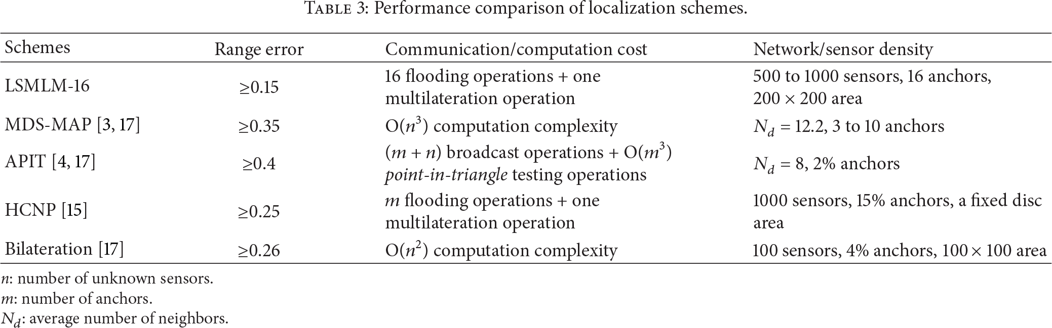
n: number of unknown sensors.

m: number of anchors.

$N_d$ : average number of neighbors.

In [15], the authors proposed a new source to destination (s2d) distance estimator known as HCNP based on the observation that there exists some correlation between the number of destination's neighbors with hop count $h\pm 1$ and the s2d-distance. The HCNP algorithm makes use of the destination's hop-count information and the information on the number of neighbors with hop count $h\pm 1$ to estimate the s2d-distance.

In [16], Cota-Ruiz et al. presented a distributed and formula-based bilateration algorithm that can be used to provide an initial set of locations. In their scheme, each node uses distance estimates to beacons to solve a set of circle-circle intersection (CCI) problems, solved through a purely geometric formulation. The resulting CCIs are processed to pick those that cluster together, and the average is then used to estimate an initial node location.

5.2. Simulation Results

The simulation environment in this study was set up as follows. The monitored region measured is 200 m × 200 m. The communication range was from 20 m to 60 m, and the sensor number was from 300 to 1000 in 100 increments. Sensors were randomly distributed in the region. The corresponding α values were selected from Table 1. Each simulation involved 50 tests, and the mean was used as the final result. All of the methods (i.e., the BLM, the LSMLM, and the DV-Hop method) were simulated using MATLAB R2012a software.

The range error is defined as the average localization errors of all of the deployed unknown sensors divided by the communication range. Figure 6 shows the relation between the true locations of the deployed unknown sensors and their corresponding estimated locations using LSMLM-16 for the case of 300 sensors and $R=40$ .

Figure 6

Illustration of true locations versus estimated locations of LSMLM-16 with 300 nodes and communication range 40 in a 200 × 200 area (red dots: true locations; red crosses: estimated locations; blue lines: connections between corresponding true and estimated locations).

Figure 7 shows the range errors of the BLM, the LSMLM-k (k = 4, 8, 12, 16), and the DV-Hop method for various communication ranges and numbers of sensors. As anticipated, under an identical CR, the range error decreases as the number of anchor nodes increases, until the number of anchor nodes reaches 16. The experimental results show that the difference of range errors between LSMLM-12 and LSMLM-16 is within 3% in all cases. This indicates that the error rate converges as the number of anchor nodes approaches 16.

Figure 7

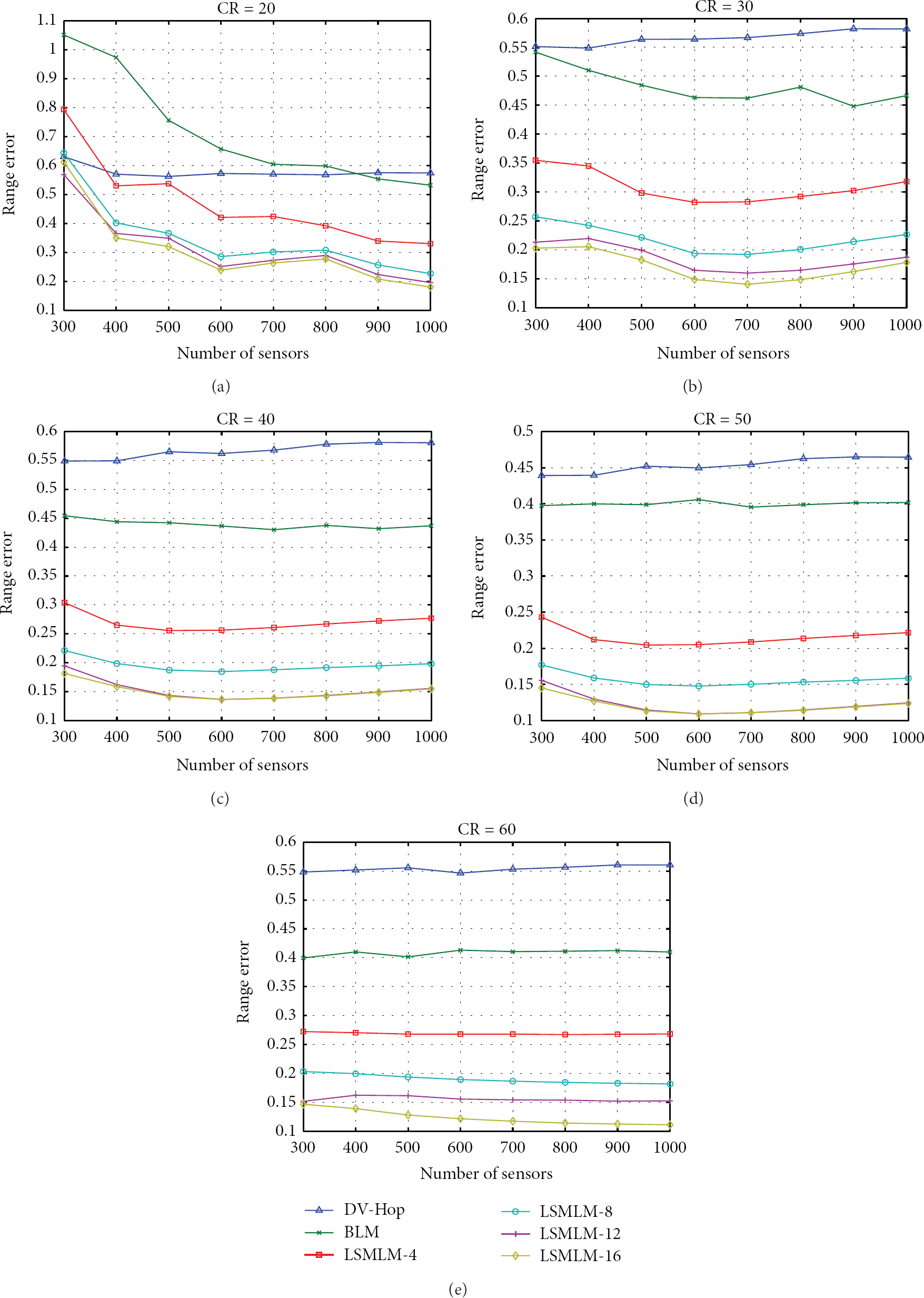
Range errors under different communication ranges (20–60 m) and node densities for BLM, LSMLM, and DV-Hop method.

Note that, in our experiments, we also used 3, 5, 6, and 7 anchors for each case of the different communication ranges. However, we found out that the error rate decreases proportionally as the number of anchors grows until the anchor number reaches 16. In order to show this observation clearly in the figures of experiment results, we only use 4, 8, 12, and 16 to demonstrate this phenomenon, instead of using the whole sequence of numbers.

For the simulation of the DV-Hop method, the percentage of anchor nodes was set to 20% since the performance falls significantly if using less than 20% of anchor nodes [2]. As shown in Figure 7, both the BLM and the LSMLM outperform the DV-Hop method, except when $\text{CR}=20$ , in which cases the node connectivity is low and each node may just have a small number of neighbors, reducing the measurement accuracy of the proposed methods. The BLM uses only two anchors, and the LSMLM uses less than 16 anchors, whereas the DV-Hop method needs to use at least 20% of the whole sensors as anchors. These simulation results indicate that the proposed scheme is more accurate than the DV-Hop method under a wide range of conditions.

Similar to the DV-Hop method, our proposed mechanism computes hop-count numbers between unknown sensors and anchor nodes to estimate the distance between them. However, our proposed mechanism is more adaptable to various situations of the distribution of unknown sensors and uses more sophisticated calculation to estimate the positions of them.

The DV-Hop method and our proposed mechanism differ in the following two aspects.

• (i)

In the DV-Hop method, each unknown sensor uses the hop size from the anchor with the smallest hop count to estimate the distances to all of the chosen neighboring anchors. The estimated distances are imprecise and usually biased according to our simulation. However, in our proposed scheme, we use (α  × hop-count number × communication range) to estimate the distances between unknown sensors and anchor nodes, where parameter α, as shown in Table 1, is derived from the prior experiments of hundreds of cases with different communication ranges.

(ii)

In DV-Hop method, each unknown sensor chooses anchors within a fixed hop count from it. These anchors may distribute unevenly, for example, gathering together or lying near the same lines of the same sides to the given unknown sensor. This will reduce the accuracy of multilateration due to the geometric dilution of precision (GDOP) [18]. However, in our proposed method, we use 16 anchors located equidistantly at the perimeter and apply the multilateration to estimate the position of the unknown sensors.

6. Conclusion

This study presents a low-cost yet effective anchor node placement strategy for the range-free localization problems of WSNs. Numerous researches have attempted to resolve the range-free localization problems in WSNs, although many of them require excessive number of anchor nodes. The proposed localization method uses as few as two anchor nodes to estimate the positions of the unknown sensors.

In this study, all anchors were installed equidistantly at the boundary of the monitored region. The distances between each unknown sensor and anchor nodes were estimated based on the minimum hop counts to the anchor nodes. The locations of the unknown sensors were derived by applying the BLM or the LSMLM depending on the number of anchor nodes. The simulation results showed that this strategy is effective. The average range error of an unknown sensor is as low as 0.15 when LSMLM-16 is employed and CR is greater than 50 meters.

The BLM uses only two anchor nodes to locate the unknown sensors. Although the BLM is appealing because of the low installation cost and communication overhead, its range error is slightly high (between 0.4 and 0.5 in general). Thus, it is suitable for coarse-grained localization. This study showed that adding more anchor nodes can reduce the error rate. The experiments also showed that the marginal effect of adding anchor nodes to reduce the error rate decreases as the number of anchor nodes increases. In the LSMLM, the error rate converges as the number of anchor nodes approaches 16.

The proposed localization scheme was compared with the established DV-Hop method. The simulation results showed that the proposed scheme surpasses the DV-Hop method in terms of localization accuracy and communication cost.

Although both the BLM and the LSMLM were applied to the monitored square region in this study, identical algorithms can be used for a rectangular region without requiring modification.