Sage Journals: Discover world-class research

Abstract

An effective new formulation is developed for simulation of transitional flows. This formulation is based on modifications made to the latest numerical model utilizing vorticity and momentum thickness Reynolds numbers concepts. In this respect, rigorous experiments were conducted in a wind tunnel to modify the existing formulation to a more reliable form suitable for modeling of transitional flows. Test model was a linear cascade of axial compressor blades. Wind tunnel tests consisted of measurements of surface pressure distributions and velocity profiles utilizing hot film anemometry. Different freestream turbulence intensities, flow incidences, and Reynolds numbers were examined. New correlations were imposed to a commercial numerical flow solver;applying them to some standard objects produced more reliable results than those obtained from other formulations, presented so far. This attribution is more emphasized especially while dealing with modeling laminar separation bubbles, where transition occurs within the free shear layer.

1. Introduction

Numerical simulation of transitional flows has gained increasing attention in the recent years. Treating transition in common approaches, like RANS method (Reynolds averaged Navier-Stokes equations), involves two major aspects of determination of its precise position and modeling the laminar to turbulent transition regions. Generally speaking, apart from simply taking measured values from experiments, approximate location of transition can be derived from empirical correlations [1].

The only transition models which are comparable with modern CFD methods can be referred to low Reynolds number ones. These models rely entirely on the capability of wall damping terms to capture the effects of transition. They are also expected to only simulate bypass transition which is dominated by diffusion effects from the freestream. Formulations of these models still exhibit a close connection between the viscous sublayer behavior and the transition calibration process. Recalibration of even one function encountered in these types of methods may change their whole performance. It is therefore not possible to introduce experimental information without a substantial reformulation of the entire model. It should be noted that although this formulation seems to be rather efficient, experimental results haveshown that other factors like freestream turbulence intensity, streamwise pressure gradient and wall roughness may affect the transition [1 –3]. As a result, damping functions could not reliably predict such a different and complex physical process alone. Therefore, they could not be widely used in industrial computational fluid dynamics simulations.

Another approach, which is rather reliable in industry, is based on experimental correlations. These correlations usually relate the freestream turbulence intensity to the momentum-thickness Reynolds number at transition onset point (Re_θt). A typical example can be referred to Abu-Ghannam and Shaw's correlation, which is based on a large number of experimental observations [4]. Although this method proves sufficiently accurate, its variables which affect production term of intermittency transport equation are local parameters. Therefore, the predictive capability of the transport equations themselves would be limited because the main inputs to the formulations are provided by experimental correlations and, in addition, physical argumentations are still needed in their derivation process.

A new theory for correlation-based models was introduced by Menteret al. in 2002 [5]. In this model, vorticity Reynolds number is introduced and used to activate the production term of intermittency equation as local information. Although Menter's initial correlation does predict and simulate the transition phenomenon rather reasonably, major revisions to his model were performed by his team in 2006 [6]. They modified correlation presented by Abu-Ghannam and Shaw [10] and Fashifar and Johnson [7] through introducing a new concept. In this respect, they corrected the correlation for intermittency term for separated flows by introducing a factor designated by γ_eff. This function helps turbulent kinetic energy factor (k) to be increased in the separated layer by changing its values to exceed over unity [6].

A new formulation is presented in this paper for simulation of transitional flows. It is based on results obtained through intensive wind tunnel tests performed on a linear cascade of axial compressor blades. Different freestream turbulence intensities, flow incidences, and Reynolds numbers were examined. Investigations were mostly focused on conditions in which a laminar separation bubble formed over the blade surface. Wind tunnel test results of the present authors, obtained from their previous investigations on a flat plate, were also used in derivation of the new correlations.

2. Laminar Separation Bubble

Laminar separation bubble may occur over different objects depending on flow properties and conditions. Occurrence of this phenomenon can considerably affect fluid dynamics performance of objects operating somehow in transitional flow regime. At low Reynolds numbers boundary layer flow may remain laminar all over the object surface. Increasing the Reynolds number may cause transition from laminar to turbulent regime to occur in the free shear layer. Since the turbulent flow is more energetic than the laminar one, flow may reattach to the surface and form a bubble. Generally speaking, transition from laminar to turbulent may depend on many factors including freestream turbulence intensity, streamwise pressure gradient, flow compressibility, wall roughness, and rate of heat transfer from the solid walls. Figure 1 shows a typical laminar separation bubble. Due to the existence of adverse pressure gradient, flow may separate from the surface, while the boundary layer is in laminar state. This point is designated by S in this figure. Transition in the free shear layer has occurred around a region, which is shown by letter T. Letter R refers to turbulent reattachment point in Figure 1.

Figure 1:

Typical laminar separation bubble.

The region on the bubble which extends from S point to T is referred to as “stationary zone” and from T to R as “circulatory zone.” Pressure distribution is nearly constant in the stationary zone, whereas it grows sharply in the circulatory part.

Separation bubbles may occur over objects located in internal or external flows. They may form on aircraft wings or bodies. They may be short or very long to cover major part of the blade surface. In internal flows they may form, for example, on compressor or turbine blades of a gas turbine engine. First stage blades of an axial compressor or axial turbine may be exposed to bubble/bubbles on their surfaces.

3. Model and Experimental Setup

Test model was a linear cascade of three blades of an axial compressor. Experiments were conducted in an open circuit blowing type subsonic wind tunnel of Aerodynamics Research Laboratory of the Iran University of Science and Technology (IUST). Figure 2 is a photograph of the wind tunnel modified for the present studies. Figure 3 shows the model installed in the wind tunnel together with hot film anemometer probe. Each blade profile was of NGTE10C4/30C50 type and was made of Plexiglas. The first two digits, 10, denote the maximum thickness in percent chord; C4 indicates a thickness distribution; 3.0 indicates camber angle in degree; C refers to the type of mean line, in this case, circular arc; and 50 is the distance of the point of maximum camber from the leading edge in percentage of the blade chord length [1]. Each blade was of 146 mm in its chord length. The cascade solidity (i.e., chord to spacing ratio) was equal to unity and its installation angle was 36 degrees.

Figure 2:

IUST linear cascade test-rig.

Figure 3:

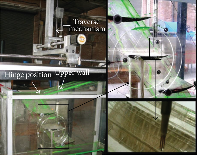
Wind tunnel test section, traversing, and anemometry mechanisms.

Almost all typical low-speed cascade tunnels discharge to the atmospheres and are powered by variable-speed centrifugal or axial blowers [5]. As has already been mentioned, the wind tunnel used in the current study was of blowing open circuit subsonic type. Honeycomb and mesh screens are mounted upstream the tunnel test section to reduce freestream turbulence level and make it uniform as much as possible. The original dimensions of the tunnel test section were 45 × 45 cm. To increase the air speed to the desired value of 52 m/s a secondary nozzle of contraction ratio of 3 was designed and manufactured and then mounted at the exit section of the original tunnel (see Figure 2). The top wall of the final test section was hinged to the tunnel solid walls to be set manually at desired angle in order to conduct the exit flow along the proper direction (see Figure 3).

Measurements were performed on the middle blade (see Figure 2). 30 pressure tappings were mounted evenly spaced all around this blade along its mid span. Pressure tappings of the test blade were connected to the pressure transducers of piezoelectric type via suitable plastic tubes. These sensors are all made by Honeywell company (model number: 162PC01D) and are ranged between 0 and 1 PSI. A suitable computerized data accusation system was used to log the surface pressures under different conditions.

Hot film anemometry was used to measure instantaneous air velocities and flow directions at proposed points. Using this type of anemometry provided to identify the flow direction. Hot film probe used through the tests consists of two parallel thin cylindrical sensors (see Figure 3). Each sensor consists of a tungsten film deposited on a ceramic cylinder (as an electrically insulating substrate) which is suspended between two prongs.

Generally speaking, hot film anemometry works on the basis of convective heat transfer from heated sensing elements. Wake flow of the upstream sensor affects the heat transfer rate of the downstream one. Consequently, it would be possible to identify the direction of the fluid flow in addition to its velocity magnitude. A servo amplifier was used to keep the temperature hence the resistance of the sensors constant. In other words, the mechanism works on the basis of constant temperature anemometry (CTA). Diameter of each hot film cylinder was 125 μm and the response frequency of anemometry was 10 KHz.

Thehot film probe was moved via a 3-degree freedom traverse mechanism which was itself controlled by a computerized system (see Figure 3). A precise ball screw mechanism provided an accuracy of 0.01 mm for any linear displacement.

Different Reynolds numbers based on the blade chord length, ranged between 80000 and 500000, were examined. The Reynolds number was varied by changing the air flow rate via a speed control mechanism attached to the tunnel driver of blower type. Flow incidences were ranged between −8 and+8 degrees with 2-degree intervals. The blades incidences were changed via coinciding their chord lines with prescaled angular positions stamped on the tunnel solid walls. Freestream turbulence intensity was changed between 1.25 and 4 percent by mounting different mesh screens upstream the test model. These flow conditions were provided to establish various flow regimes, in terms of fully laminar and transitional flows, over the blade surface.

4. Numerical Formulation

Transport equation for intermittency γ function can be used to capture transition phenomenon locally. This function can be coupled with SST k-ω based turbulence model to trigger the transition point by activating the production term of the turbulent kinetic energy downstream of the transition point [9]. Formulation of the intermittency has also been extended to account for rapid onset of transition caused by separation of laminar boundary layer. In addition, the model can be fully calibrated for proper prediction of both the transition onset point and its extent.

Second transport equation is introduced based on momentum-thickness Reynolds number at transition, Re_θt. This transport equation plays a significant role for activating the transition, since it is originally calibrated based on the experimental results. More information about this method can be obtained by referring to the paper published by Menter et al. [6].

In the following sections, initially, modifications to the original model are introduced in order to recover its deficiency in simulation of separated flow transition. Then, new empirical correlations, which are obtained by the present authors, are introduced for improvement of the correlations presented by Menter et al. [6].

New empirical correlations presented in the following sections are all based on results obtained through extensive tests carried out by authors on the model introduced in the previous section. As has already been mentioned, a linear cascade of axial compressor blades were tested in a proper wind tunnel, usinghot film anemometry and surface pressure measurements provided to obtain the flow properties in details. Postprocessing of experimental results included calculations of the boundary layer parameters and those relevant somehow for describing the characteristics of the transitional flows.

4.1. Newly Developed Correlations for Separated Flows

One of the main deficits of the original model is about simulation of separated flow transition. Whenever the laminar boundary layer separation occurs, using original model predicts the possible reattachment point too far downstream than it may occur in reality. In addition, it may predict position of separation point which is not consistent with experimental results. This disagreement with experimental data tended to increase as the freestream turbulence intensity was lowered [8]. The reason is mostly based on the behavior of turbulent kinetic energy (k) in separated flows which could not increase large enough to cause possible reattachment of the separated boundary layer. So, the way to trigger better the reattachment is to force k factor to grow. It would be possible through changing the intermittency factor to exceed over 1 whenever the laminar boundary layer separates. This procedure will result in a large production of k, which, in turn, will cause earlier reattachment of the separated flows.

A correlation-based transition model is introduced by Menter et al. using local variables [6]. Their results are presented in Figure 4. As it is apparent from this figure, when the laminar separation occurs, the vorticity Reynolds number Re_ν, significantly exceeds the critical momentum thickness Reynolds number, Re_θc. Therefore, the ratio between these two Reynolds numbers can be thought as a measure of the size of the laminar separation and can therefore be used to increase the production term of the turbulent kinetic energy [6].

Figure 4:

Relative error between vorticity Reynolds number and momentum thickness Reynolds number as a function of boundary layer shape factor [6].

The modified version of governing equations, developed by the present authors for separation-induced transitional flows, is presented as follows:

γ_{sep} = \min {s_{1} \max [\frac{R e_{ν}}{3.145 R e_{θ c}} - 1] F_{reattach}, 5} F_{θ t}, S_{1} = 6,

(1)

where,

F_{θ t} = \min (\max (F_{wake} \cdot e^{- {(y / δ)}^{4}}, 1.0 - {(\frac{γ - 1 / c_{e 2}}{1.0 - 1 / c_{e 2}})}^{2}), 1.0), C_{e 2} = 50,

(2)

F_{reattach} = \frac{(- 2.5 e - 6) + 1.056 R_{T}^{- 3.583}}{(1.14 e - 4) + R_{T}^{- 3.583}},

(3)

γ_{eff} = \max (γ, γ_{sep}) .

(4)

Differences between the present model and Menter's modified model [6] lay on the ratio of Re_ν to Re_θc, F_reattach, and constant S₁. Generally speaking, the size of the separation bubble can be controlled by constant S₁. F_reattach checks the viscosity ratio and when it is large enough, it causes reattachment to occur. The blending function F_θt is used to turn off the source term in the boundary layer and allow the transported scalar $\bar{R e_{θ t}}$ to diffuse in from the freestream. F_θt is equal to zero in the freestream and is equal to one within the boundary layer. F_wake function ensures that the blending function is not active in the wake regions downstream of the obstacle. The dissipation term manages k factor so that it can never exceed its relevant fully turbulent value.

4.2. New Correlations for Re_θt

Suzen et al. [3] have shown that for a low-pressure turbine blade exposed to a high turbulence intensity inflow the correlation of Abu-Ghannam and Shaw [10] results in transition onset being predicted before the laminar boundary layer to separate. As a result, the possible separation bubble on the suction side of the blade would be too small. In the correlation presented by Abu-Ghannam and Shaw [10] transition onset momentum thickness Reynolds number, Re_θt, does not vary when the flow is strongly accelerated. Nevertheless, as is shown by Suzen et al. [3] through their experiments, strong accelerations can result in significant increase in Re_θt.

The correlation of Abu-Ghannam and Shaw [10] does predict transition in zero and negative pressure gradient flows, well. It would therefore be of great attraction to have an empirical correlation which behaves similar to that of these researchers for flows which cover all kinds of zero, positive and negative pressure gradients. In this respect, comprehensive attempts have been carried out by present authors to enhance the Re_θt empirical correlation for natural and bypass transition mechanisms.

New correlations obtained in the present research work are basically an adaptation of Abu-Ghannam and Shaw's postulation. They have proposed that Re_θt could be interpreted as a cross product of two functions introduced by F(λ_θ) and Re (Tu). F(λ_θ) is itself a function of Tu and λ_θ, and Re (Tu) is defined only for zero pressure gradient case. The following describes how these two functions are obtained based on the experimental works of the present authors.

Figure 5 shows variations of Re_θt with Tu for zero pressure gradient case (λ_θ = 0). These results include previous experimental data of the present authors, Fashifar and Johnson [7] and Abu-Ghannam and Shaw [10]. Curve fitting on the whole results, shown by a solid line in Figure 5, produced the following correlations valid for zero pressure gradient case:

\begin{matrix} {Re}_{θ t} = 1099.3 (0 . 5^{Tu}) ({Tu}^{- 0.1}) ⟹ Tu \leq 1.6, \\ R e_{θ t} = 467.62 {Tu}^{- 0.761} ⟹ Tu ≻ 1.6 . \end{matrix}

(5)

Figure 5:

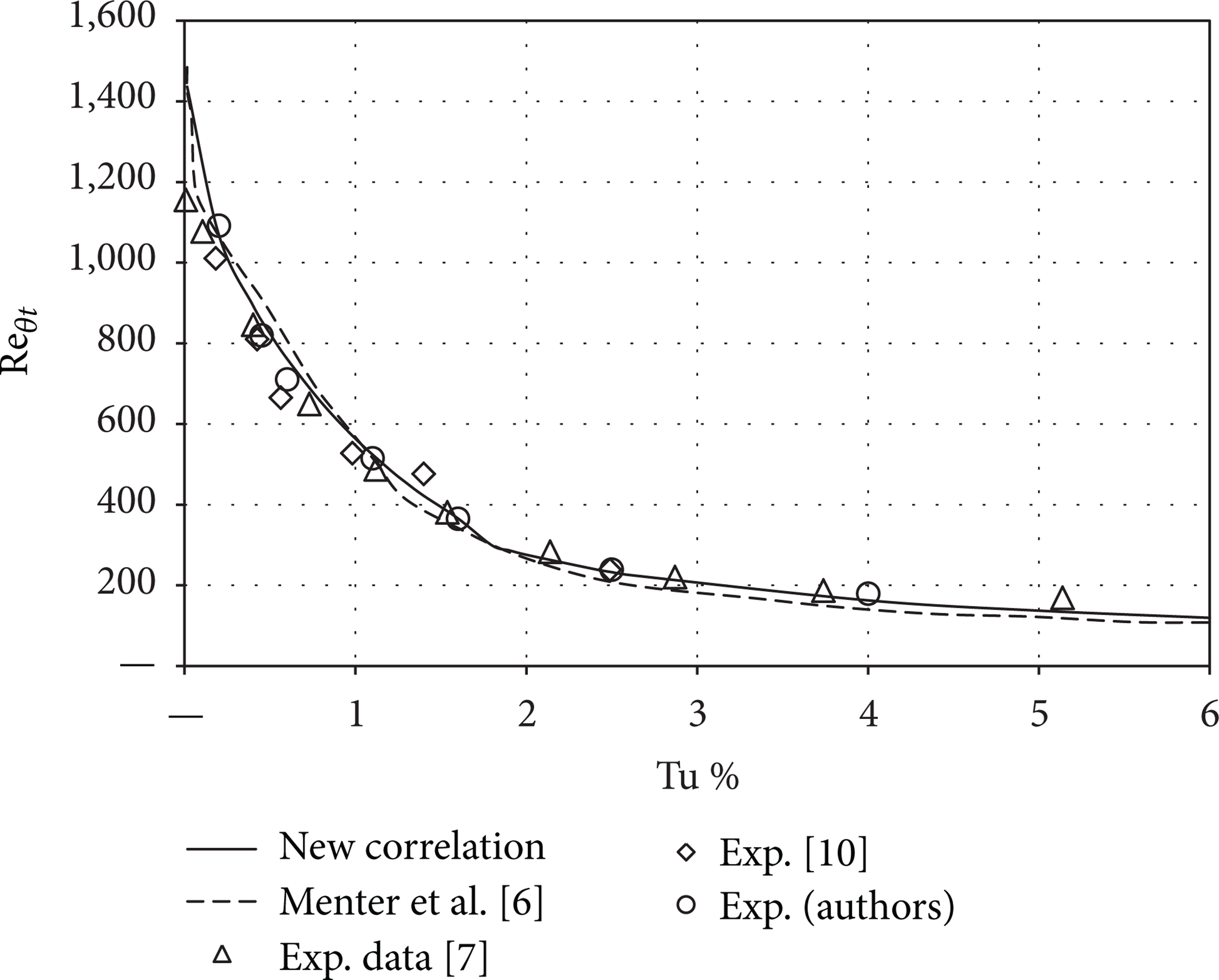
Variations of Re_θt with turbulence intensity.

Results of correlation presented by Menter et al. [6] are also superimposed in Figure 5.

Wind tunnel test results of the present authors on their models are provided to obtain F function as follows:

\begin{matrix} F (λ_{θ}) = 1 - (- 6 λ_{θ} + 25.5 λ_{θ}^{2} + 10 \cdot λ_{θ}^{3}) \cdot e^{- [Tu / 4]}, λ_{θ} \leq 0, \\ F (λ_{θ}) = 1 + 0.556 (1 - e^{- 40 λ_{θ}}) \cdot e^{- [2.5 Tu]}, λ_{θ} ≻ 0 \\ - 0.1 \leq λ_{θ} \leq 0.1, \\ Tu \geq 0.027, R e_{θ t} \geq 20 . \end{matrix}

(6)

To a certain extent, close agreements can be observed between all results shown in Figure 5. However, it will be shown in the following sections that correlations presented by the present authors are more accurate than those proposed by other researchers. At low turbulence intensities, the new correlation has been designed to predict a large increase in Re_θt whenever a favorable pressure gradient is present. Based on the Fashifar and Johnson [7] data, the effect appears to reduce as the freestream turbulence intensity increases. Authors' new correlation is also designed somehow to reflect this fact.

Variations of Re_θt with pressure gradient parameter λ_θ are shown in Figure 6 for different turbulence intensities. Some researchers like Susan et al. [3] believe that Abu-Ghannam and Shaw's [10] correlations do not work well within the positive pressure gradient and flows with very low turbulence intensities. In these types of flows the commencement point of transition ispredicted earlier while using the correlations presented by these latter researchers. Present authors claim that their new correlations can recover this deficiency. These new correlations predict results in close agreement with those of Abu-Ghannam and Shaw in negative pressure gradient zones and for turbulence intensities of greater than 0.3%. However, although for Tu values less than 0.3% discrepancies between results get larger, it is worth mentioning that those obtained by the present authors are very close to the experimental data. This consistency can be detected for all the Tu values, especially for the authors' lowest test case of 0.03% (specifications of this latter test case is introduced in Table 1).

Table 1:

Test cases [1, 2].

Test case	μ/μ_t	U (m/s)	Tu (%)	μ/μ_t

T3A	10	5.2	3.8	10
T3B	40	9.4	6.5	40
T3C4	5	1.4	3	5
Zierke blade (PSU)	1	32.9	0.18	1
Flat plate (Authors)	20	15.5	0.03	20

Figure 6:

Variations of Re_θt with pressure gradient parameterλ_θ.

4.3. New Correlations for Re_θc

Re_θc is the critical Reynolds number where the intermittency first starts to increase in the boundary layer. Re_θc corresponds to the position prior to the point of transition (with corresponding Reynolds number Re_θt), since there is a delay for turbulence intensity to grow and reach its appreciable levels necessary for commencement of transition [6]. As a result, Re_θc can be thought as a criterion for prediction of the position where the turbulence spots starts to grow. On the other hand, Re_θt refers to the location where the velocity profile first starts to deviate from a purely laminar profile, indicating the commencement of transition. The relation between these two Reynolds numbers could be interpreted by a suitable empirical correlation. Based on previous wind tunnel tests of the present authors performed on a flat plate, there is a linear function between these two parameters, which is introduced by

R e_{θ c} = f (\overset{—}{R e_{θ t}}) = 0.5086 \overset{—}{R e_{θ t}} + 65.118 .

(7)

4.4. New Correlations for F_Length

The production term in intermittency transport equation is designed to be equal to zero in the laminar boundary layer upstream of transition point and to be activated everywhere the local vorticity Reynolds number exceeds its value at transition onset. The magnitude of this source term is controlled by the transition length function (F_Length) [6]. In other words, F_Length is an empirical correlation which controls the length of the transition region.

New correlations for F_Length are obtained through combination of ERCOFTAC's results [1, 2] and experimental results of the present authors already performed on a flat plate. In addition, current authors' experimental results obtained for their model (a linear cascade of axial compressor blades of NGTEC4 type) were used for tuning this new correlation.

Since the ERCOFTAC data correspond to bypass transition related to moderately low to high turbulence intensities, the natural transition data of the authors and those of Menter et al. [6] were used to calibrate the new correlation for F_Length. The final form of the newly developed correlations is presented as (8) and their graphical interpretation is shown in Figure 7:

\begin{matrix} F_{Length} = e^{65 - 1185 / R e_{θ t} - 10.2 Ln (R e_{θ t})} ⟹ 180 ≺ R e_{θ t} ≺ 600, \\ F_{Length} = 0.55 ⟹ R e_{θ t} \geq 600, \\ F_{Length} = 300 ⟹ R e_{θ t} \leq 180 . \end{matrix}

(8)

Figure 7:

Variations of F_Length with Re_θt.

Using this function revealed the fact that F_Length values are small for large amounts of Re_θt (i.e., low turbulence intensities) and vice versa. Furthermore, the solution is rather insensitive to F_Length for small values of Re_θt (i.e., high turbulence intensities).

It should be noted that the Re_θc and F_Length correlations are strong functions of each other and significant amount of iterations are required in order to obtain a reasonable consistency between them.

5. Validation of the New Empirical Correlations

The well-known transitional test cases of ERCOFTAC [1, 2] T3 series, which are usually used as the benchmark for transitional flow studies, are used to examine and validate the new model. Zierke blade (PSU), corresponding to Deutsch Compressor Cascade [8], is also tested to approve the capability of the new correlation in modeling the transitional flows. These test cases, including various flow conditions, are introduced in Table 1.

The first two cases of T3A and T3B belong to zero pressure gradients with freestream turbulence levels of 3.8% and 6.5%, respectively, which correspond to transitional flows of bypass type. T3C4 test case corresponds to the flow in the presence of a separation bubble. This latter test case is considered in the present study to reveal the capability of the new model for prediction of separation induced transition and the subsequent reattachment of the turbulent boundary layer.

Figures 8, 9, and 10 show the variations of skin friction coefficient with Reynolds number for T3A, T3B and T3C4 test cases. Results of Menter et al. [6] are superimposed in these figures for comparison. Close agreements between the results of the present model with those of the experimental data are obvious. These satisfactory consistencies prove the capability of the present model for prediction of the location of transition and variations of flow parameters in pre-transitional and turbulent regions.

Figure 8:

Variations of skin friction coefficient with Reynolds number for T3A test case.

Figure 9:

Variations of skin friction coefficient with Reynolds number for T3B test case.

Figure 10:

Variations of skin friction coefficient with Reynolds number for T3C4 test case.

The portion of curves laid under zero skin friction coefficient line in Figure 10 indicates the occurrence of a laminar separation bubble.

Numerical results of the present authors' model and those of Menter et al. formulation, obtained for Zierke Deutsch Compressor Cascade (PSU), are shown in Figure 11. Experimental results of Zierke compressor are also superimposed in this figure for comparison. Close agreement between the new correlation results with experimental data of Zierke, especially in capturing the laminar separation bubble (domain of negative C_f values), can clearly be detected in this figure.

Figure 11:

Skin friction coefficient distribution for the Zierke (PSU) compressor blade [8].

6. More Results of the Test Model

The computational domain and boundary conditions are shown in Figure 12 for the test model (i.e., NGTE10C4/30C50 blade). The grid structure consisted of 1600000 cells. Both the blade pressure and suction sides had a viscous sublayer grid type with a maximum y+ of unity. Grid independency studies were carried out and showed no significant variations in the results for mesh numbers exceeding the above-mentioned value.

Figure 12:

Computational domain and boundary conditions for NGTE10C4/30C50.

In the previous sections new correlations were obtained for modeling transitional flows utilizing authors own wind tunnel tests. Then, these correlations were validated via comparing corresponding results with those obtained by other researchers and those extracted from the authors own tests. This section is devoted to presentation of more results obtained through the authors' wind tunnel tests and those obtained through their new correlations.

Figures 13 and 14 show distributions of surface pressure and skin friction coefficients, respectively. The most important feature of these results is the high capability of the newly developed transitional model in predicting the occurrence of laminar separation bubble on the blades surfaces under various conditions. The bubble position, designated by S.B. in pressure results, is recognized by initial level pressure distribution followed by its sudden increase. Generally speaking, the size of the separation bubble is a complex function of the freestream Reynolds number, turbulence intensity, and incidence. In principle, the newly formulated transitional model predicts the major parts of the flow precisely, that is, laminar, turbulent and transitional regions on the blades surfaces.

Figure 13:

Surface pressure coefficient distribution at different freestream turbulence intensities, incidences, and Reynolds numbers.

Figure 14:

Skin friction coefficient distribution at different turbulence intensities, incidences, and Reynolds numbers.

An important issue to note is the effect of streamwise grid resolution on resolving the leading edge laminar separation and subsequent transition on the suction side. If the number of streamwise nodes clustered around the leading edge is too low, the model cannot resolve the rapid transition and a laminar boundary layer could be resulted the suction side. For the present study, 110 streamwise nodes have been distributed between the leading edge and an axial position of 20% blade chord length.

Locations of separation and reattachment points as a function of Reynolds number are shown in Figure 15 for the model at zero incidence and 1.25% freestream turbulence intensity. It can be observed how increasing the Reynolds number has caused the bubble length to decrease.

Figure 15:

Variations of separation and re-attachment points with Reynolds number at zero incidence.

Results of Menter original model are superimposed in Figure 15. It is obvious that this model has not been able to enforce the flow to reattach to the surface.

Variations of the loss coefficient with incidence for two freestream turbulence intensities and a Reynolds number of 300000 are shown in Figure 16. It can be observed how well the losses, calculated based on the new correlations, follow the experimental results.

Figure 16:

Loss variations versus incidence at different freestream turbulence intensities, Re = 300000.

7. Conclusions

The main conclusions which can be drawn from the present research work can be stated as follows.

New correlations are capable of predicting all kinds of transitional flows over various objects better than available models presented so far.

New correlation proposed for intermittency parameter at separation point causes more production in turbulent kinetic energy term and, as a result, enforces separated flow to reattach to surface at position consistent with experimental results.

New correlation for F_Length in triggering of transitional region shows a better controlling process of source term magnitude in intermittency transport equation in comparison to existing original model.

Experimental results show that loss coefficient increases by increasing freestream turbulence intensity from 1.25% to 2.5% which is accompanied by existence of a laminar separation bubble. These results agree well with results obtained from newly developed correlations.

Incidence at which loss is a minimum is highly dependent on freestream turbulence intensity level.

Laminar separation bubble is well modeled by modifications made to original model in prediction of its total length and also location of transition within free shear layer.

Footnotes

Nomenclature

References

Savill

A. M.

, “Some recent progress in the turbulence modelling of by-pass transition,” in Near-Wall Turbulent Flows, So

R. M. C.

Speziale

C. G.

, and Launder

B. E.

, Eds., p. 829, Elsevier, New York, NY, USA, 1993.

Savill

A. M.

, “One-point closures applied to transition,” in Turbulence and Transition Modelling, Hallbäck

, Ed., pp. 233–268, Kluwer, Dordrecht, The Netherlands, 1996.

Suzen

Y. B.

Huang

P. G.

Hultgren

L. S.

, and Ashpis

D. E.

, “Predictions of separated and transitional boundary layers under low-pressure turbine airfoil conditions using an intermittency transport equation,” Journal of Turbomachinery, vol. 125, no. 3, pp. 455–464, 2003.

Langtry

R. B.

and Sjolander

S. A.

, “Prediction of transition for attached and separated shear layers in turbomachinery,” AIAA Paper AIAA-2002-3643, 2002.

Menter

F. R.

Esch

, and Kubacki

, “Transition modelling based on local variables,” in Proceedings of the 5th International Symposium on Turbulence Modeling and Measurements, Mallorca, Spain, 2002.

Menter

F. R.

Langtry

R. B.

Likki

S. R.

Suzen

Y. B.

Huang

P. G.

, and Völker

, “A correlation-based transition model using local variables—part I: model formulation,” Journal of Turbomachinery, vol. 128, no. 3, pp. 413–422, 2006.

Fashifar

and Johnson

M. W.

, “An improved boundary layer transition correlation,” ASME Paper ASME-92-GT-245, 1992.

Zierke

W. C.

and Deutsch

, “The measurement of boundary layers on a compressor blade in cascade, vols. 1 and 2,” NASA CR 185118, 1989.

Wilcox

D. C.

, Turbulence Modeling for CFD, DCW Industries, La Canada, Calif, USA, 1993.

10.

Abu-Ghannam

B. J.

and Shaw

, “Natural transition of boundary layers—the effects of turbulence, pressure gradient, and flow history,” Journal of Mechanical Engineering Science, vol. 22, no. 5, pp. 213–228, 1980.