
Abstract
Two-feet climbing robot is proposed for rotor blade surface damage detection. The penalty function is designed based on the simulated annealing neural network for waypoints inside blade. According to the derivative of path energy function to time, waypoints are updated and move toward the direction reducing the path energy consisting of length and penalty function. According to the curvature variation range, a novel weighted simulated-annealing-temperature updating method is designed to get comprehensive optimization of the path energy and convergence speed. The path planning is accomplished for the root, middle, and tip blade parts, respectively. The asymptotic analysis of the waypoint coordinating updating process was given, and the updated start point is adopted during escaping from inside. The effect of weight on path energy and convergence speed is analyzed. The planning results show the effectiveness of the proposed path planning algorithm, and the weighted average method is valid for the comprehensive optimization.
1. Introduction
Bearing the huge wind stress during energy conversion process, the rotor blade is among the most easy-to-failure components of wind turbine generator system (WTGS) [1]. Due to that blades are vulnerable to cumulative fatigue damage owing to the periodic nature of the loading, detecting damage to blades before failure is crucial. Currently, rotor blades damage is only detected manually, which is dangerous and low effective. The authors propose to use the climbing robot to detect blades surfaces damage.
Aiming to find an optimal path from start to target point in an unstructured environment, the path planning is one of the fundamental problems in robots detecting surface automatically. The path planning can be classified into two major categories, global and local path planning, according to the environment information [2–4]. The global path planning creates a path in a static environment, while the local path planning does in a dynamic environment. Due to the dynamic obstacles, the obstacle avoidance method is the key in the local path planning, such as the virtual force field, Elman fuzzy adaptive control [5]. Owing to lack of complete environment information, local path planning algorithm is more complex than global path planning algorithm, but the latter requires the environment modeling and path searching. The literature shows that researchers have studied the visibility graphs method [6], free space method [7], topological method [8], and grid method [9] for environment modeling. These methods are mainly applied to two-dimension (2D) space.
We study the path planning for the three-dimension (3D) curved solid, and rotor blade mathematical expressed equation is more difficult. To detect blade surfaces, the climbing robot should move along the rotor blade surfaces. To this day, researchers have used the mixed integer linear programming algorithm (MILP), ant colony optimization and neural network (NN) to study the path planning method for the climbing robot in 3D space. The MILP-based path planning for city-climber robot is complex and the path length is not considered as a constraint condition [10]. Hu and Cai have presented an improved ant colony algorithm to study the mobile robot path planning in 3D space with the given environment information [11]. This algorithm's shortcoming is being time consuming and not suitable for the path planning on the surface of curved solids. Neural network is biologically inspired and robust to time-varying delay [12]. Yu et al. have proposed an aggressive algorithm based on the energy function using the artificial NN to describe the obstacles [13, 14], but this algorithm is not fit for the nonlinear boundary surfaces. Yang and Meng studied a dynamic collision-free trajectory generation using NN to avoid concave U-shaped obstacles [15]. For concave objects minimum distance problem, Carretero and Nahon designed the simulated annealing (SA) and genetic algorithms (GAs) [16]. Blade includes both the convex and concave; therefore, the path planning for the minimum distance is more complicated problem. For the stability of NN, the weighting method is valid, and Zhang et al. gave a solution based on optimization method to calculate the optimal weighting-delay parameters [17].
To the best of our knowledge, there still is not a suitable path planning for robot climbing on the blade surfaces of wind turbine. This paper studies a 3D space path planning method for rotor blade climbing robot based on the artificial neural network and simulated annealing described in [18]. The main contribution of this paper is to extend the NN path planning from linear boundary to nonlinear boundary surfaces including both convex and concave in 3D. Meanwhile, the weighted average of SA temperature is designed to improve the comprehensive performance of the planning speed and the path length. Furthermore, the weight formulation is designed according to the surface's curvature.
This paper is organized as follows. In Section 2, we firstly give the climbing robot prototype and analyze the curvature varying of blade. The penalty function between waypoints and 3D curved solids is designed based on artificial neural network. Path energy function is defined and waypoints moving directions are derived. The weighted calculation of the simulated annealing temperature is proposed for the comprehensive optimization of path energy and convergence speed. In Section 3, we give the detailed parameters of path planning. Simulations on whole blade are conducted and the annealing temperature weight adjustment is done to illustrate the significance of proposed weight formulation. Computing results are shown at the end of Section 3. The conclusion is drawn in Section 4.
2. Path Planning Design Using Neural Network
2.1. Climbing Robot Prototype and Rotor Blade Curvature
We have developed a climbing robot for blade damage detection shown in Figure 1. We combine climbing techniques with a modular approach to realize a practical climbing robotic based on an easy-to-build mechanical structure [19]. This robot has two feet and three degrees of freedom, and each foot has three vacuum suckers installed in the vertex of a triangle. All joints are actuated by DC servomotor. The robot mechanical structure consists of foot modules (Joint 1 and Joint 2) and body module (Joint 3). Through adding the foot or body module, we can get the more flexible caterpillar-climbing robot expediently. This robot can climb rotor blade surfaces with swing-around gait and carry the camera, ultrasonic or infrared instrument to detect the blade.

The mechanism and snapshots of climbing robot on the wind turbine blade: (a) the mechansim sketch; (b) the snapshots.
This two-feet climbing robot has light weight and only two interaction contact areas with blade surface, so it can be more easily adaptive to varying curves than climbing robot with more feet. In path planning, the robot can be simplified as the two-link mechanism. The Joint 2 at the center of mass or shape connects two links, and the end of each link is the foot. The planned path is composed of a number of waypoints between start and target point. These waypoints mean the continuous footprints.
It is difficult to express the whole rotor blade accurately by mathematical equations, so we divide the rotor blades into three parts according to the curvature, as shown in Figure 2.
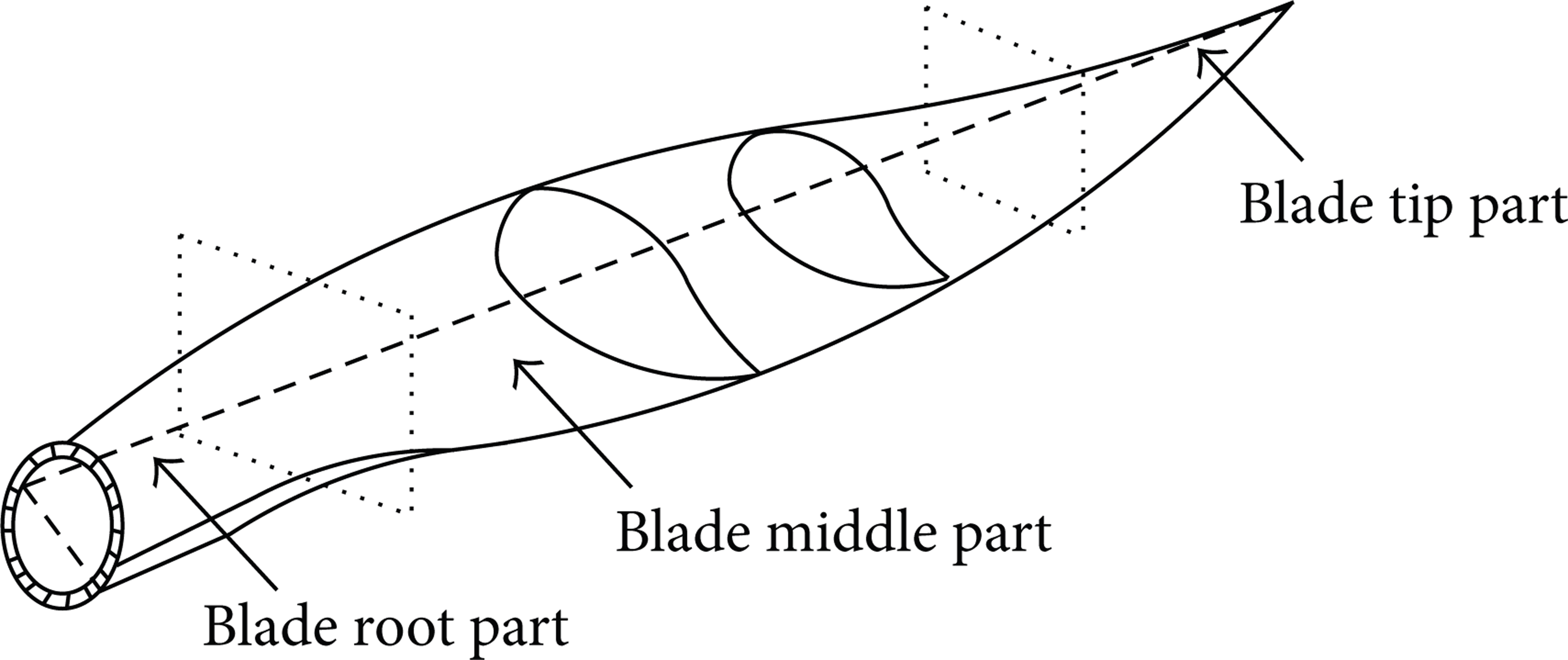
Division of rotor blade.
According to [20], we properly idealize the curvature variation range of each part shown in Table 1. The curvature variation range of root part is very small, so we model this part as a cylinder. The curvature variation range of middle part is relatively large, so we model this part as a polyhedron surrounded by regular curved surfaces. The tip part is modeled as an elliptic cone.
Parameters of the rotor blade.

For climbing motion, footprints should be on the blade surface proper, so we should punish these waypoints under or out of blade surface.
2.2. Penalty Function of Point Based on Artificial Neural Network
Penalty function method is usually used to solve the constrained minimization problems. The key point of this method is to obtain an augmented objective function by adding a penalty function to the original objective function. Namely, penalty function should add a great penalty value to these points attempting to cross the border or escape from the feasible region. In this paper, we define the path penalty function as the sum of all waypoints' penalty function. The value of each waypoint penalty function is obtained using the artificial neural network shown in Figure 3.

Artificial neural network of a waypoint's penalty function.
Three nodes in input layer denote the x,y, and z coordinate values of the given waypoint in the Cartesian. The boundary surface is defined as F m (x, y, z) = 0, and then constraint equations of the given blade curved solid can be shown as

where M denotes the count of boundary surfaces of the given blade sector.
In the Interlayer 1 and Interlayer 2, the count of nodes is equal to M. Moreover, the value of node connection weight between input layer, interlayer, and output layer is set to 1 specially.
Input and output of above artificial neural network nodes are


where I m and O m are the input and output of node m in the Interlayer 2, respectively; I o is the input of the node in the output layer; C i is the output of the node in the output layer, namely, the penalty function value of waypoint P i (x i , y i , z i ); θ I is the threshold of the node in output layer; N is the count of discrete waypoints that depends on the climbing step length and the sizes of robot mechanism. Excitation functions of the nodes in the output layer and Interlayer 2 adopt S type Sigmoid functions as follows:
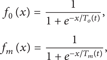
where T0(t) and T m (t) are the annealing temperature varying with time t.
Define the value of the whole path penalty function as

where C i is between 0 and 1, which reflects the collision risk between the waypoint and the curved solid.
2.3. Path Energy Function and Planning Algorithm
Path energy function is used to represent the energy consumption of robot climbing along the given path. We define the path energy as the sum of the path length and penalty function
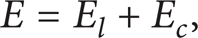
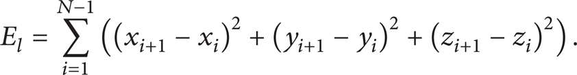
where E l represents the sum of square of each segment length L i (L0 = L N = 0),
Waypoints should move towards the direction decreasing the path energy. Namely, waypoints should move from the inside to curved solid surfaces, and the path length should be restrained as short as possible.
We formulate the derivative of the energy function to time and get
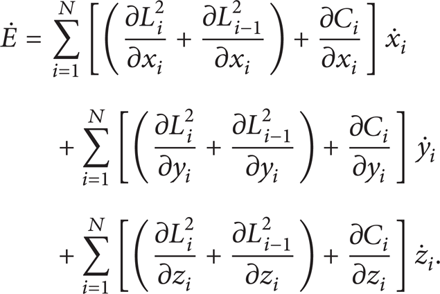
Define

where η1 is a positive constant that denotes the optimizing rate of energy function.
Substituting equation set (9) into (8), we can get

So equation set (9) can ensure that waypoints are moving towards the direction decreasing the path energy.
Then by substituting (3) and (7) into equation set (9), we get the dynamic planning equation of waypoint P i (x i , y i , z i ) as follows:

The previous section of equation set (11) is used for optimizing the path length, while the latter section is used for making waypoints to move from curved solid inside to surfaces. So waypoints within the curved solid should move according to equation set (11).
For waypoints on the curved solid surfaces, the latter section of equation set (11) is unnecessary, so these waypoints should move according to the equations as follows:

where η2 is a positive constant denoting the optimizing rate of path length.
Equation set (11) and (12) indicate the rough and careful adjustment of a waypoint location, respectively. So we usually set η1 > η2 in the path planning algorithm.
2.4. Temperature Updating Using Simulated Annealing
The energy function above may have multiple extremum values, as a result, and the path planning algorithm may fall into local minimum points quickly. In order to escape from the local minimum problem as far as possible, we applied simulated annealing method to change the value of T o (t) and T m (t). Due to that the climbing robot must cost energy to adhere to the blade even in static state, the planning time and path length are coequally important. The global minimum without considering convergence speed is not practical.
Table 2 summarizes and compares the existing temperature updating functions about simulated annealing methods in the literature. Table 2 compares three main performances including the probability of escaping from local minima, the convergence speed, and the correlation with variable dimension of optimization objective.
Performances comparison of different temperature updating functions.

For online path planning, we want to design a temperature updating function that can escape from local minimum as far as possible and enhance convergence speed to reduce the planning time simultaneously.
Design T o (t) and T m (t) as follows:

where α is the weight, and β0 and β m are the initial simulated annealing temperature in the output layer and Interlayer 2, respectively.
Curvature of boundary surfaces is not been considered in the past literature. Intuitively, the path planning is easy to fall into the local minimum due to large varying range of curvature, so in this case we should increase α to reduce the speed of temperature change. Therefore, in flat surface, α should be less for quick convergence, while in curve surface, α should be larger for escaping from local minima. Therefore, the surface curvature variation is the key to setting α value. We creatively design α as the following formulation:
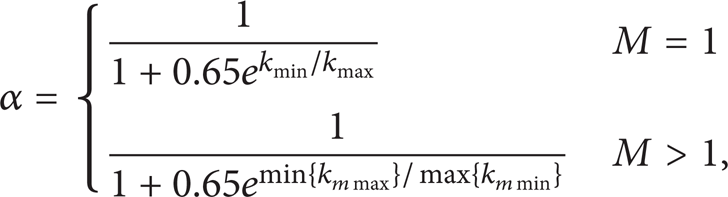
where k mmin and k mmax denote the minimum and maximum curvature of the m boundary surface, respectively.
2.5. Path Planning Processing
We assume that start point P(x1, y1, z1) and target point P(x N , y N , z N ) are located on the curved solid surface. Design the path planning processing as follows.
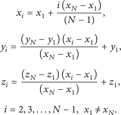
Step One. The initial path is composed of evenly distributed waypoints along the straight line between start and target point, and the waypoints coordination equations are
Step Two. If I m > 0 (m = 2,3, …, M), then waypoint P(x i , y i , z i ) is inside the curved solid and should move according to equation set (11); otherwise, P(x i , y i , z i ) is outside the curved solid and should move according to Equation set (12). Repeat Step two until all waypoints are outside the solid.
Step Three. Repeat moving all waypoints according equation set (12) until the path energy function converges to the minimum. In this paper, converge condition is defined as the changing of the path energy value is always less than 10−5 in ten cycles continuously.
Figure 4 shows the algorithm flow chart.

Flowchart of path planning algorithm.
3. Path Planning Experiments
3.1. Planning Condition
For validating the effect of the proposed path planning algorithm was implemented using MATLAB2009b on a personal computer (PC) with Intel(R) Core(TM) 2 Duo T5450 @ 1.66 GHz CPU. The Runge-Kutta method was adopted for solving equation set (11) and (12).
The rotor blade for test is shown in Figure 2. For practical computing, we established simply the constraint equations of each part based on Table 1. Constraint equations of boundary surfaces for the blade root, middle, and tip parts are shown in (16) successively. Consider

3.2. Path Planning Simulation Study
Planning experiments for each part were conducted.
Figure 5 presents the neural network of the penalty function between waypoint P(x i , y i , z i ) and blade root part. Figure 6 gives the path planning result on the boundary surfaces of root part. In Figure 6, “s” means the start point, and “g” means the target point.

Neural network between the given waypoint and blade root part.

Path planning result on the surface of blade root part.
The value of α is set to 0.36 according to the curvature variation range in Table 1 and (14). Other parameters are as follows:
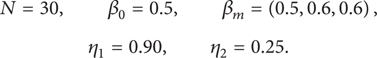
For path planning on the boundary surfaces of middle part, the simulation parameters are as follows:
The value of α is set to 0.57 according to the curvature variation range in Table 1 and (14).
Figure 7 presents the process of path planning on the blade middle part. K denotes the number of the algorithm loops.

Path planning processing of the algorithm on middle part: (a) initial state; (b) K = 35; (c) K = 40; (d) K = 71.
Figure 7 shows that the proposed planning algorithm is conducted in turn on different boundary surfaces. Furthermore, we found that waypoints orderly escaped from curved solid inside to surfaces according to the sequence from start to goal point. Although, all waypoints on the path were updated on each iterative planning, from start to goal point. Therefore, this path planning is asymptotic and all waypoints on the path are updated on each iterative planning. Meanwhile, we foundthe coordinate varying is tiny and less than 0.01 m after waypoints arrived on surfaces. So we designed a quick planning algorithm for Step two to reduce the computing burden, through updating the new start point using the waypoint just moving to the surface. However, this updating is only for Step two. When the algorithm flows into Step three, the start point should be returned to original start point. The quick planning for Step two is shown in dotted line frame in Figure 4. Planning experiments show that the computing time is 4.07 s without and 2.81 s with updating the start point, respectively.
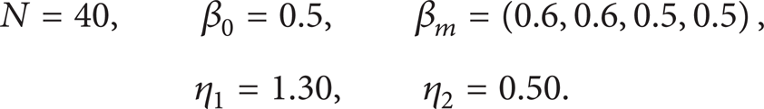
For path planning on the boundary surfaces of tip part, the simulation parameters are the following:

The value of α is set to 0.59 according to the curvature variation range in Table 1 and (14).
Figure 8 presents the path planning results on boundary surfaces of tip part.
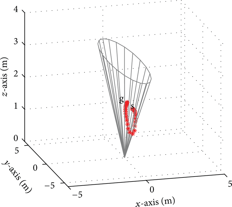
Path planning result on the surface of blade tip part.
Figures 6, 7, and 8 show the effect and success of the proposed algorithm on whole rotor blade boundary surfaces.
3.3. Annealing Temperature Weight Adjustment
Experiments on the whole blade with different α were conducted to demonstrate the performance of the proposed annealing temperature weight in (14) and (15). E and Kc denote the energy function value and convergence speed in Step two of algorithm flow, respectively.
Figure 9 shows the value of E and Kc varying with annealing temperature weight with step 0.05 in the range 0–1. The convergence speed Kc increases monotonically with increasing α in Figures 9 (a) and 9 (b), and nearly increases monotonically in Figure 9 (c). However, the energy function E decreases non-monotonically with increasing α in all Figure 9. The value of α calculated from (14) is at or close to the comprehensive optimum point for the energy and convergence speed, namely, the intersection point of two curves.

The relationships between the energy function and convergence speed with weights: (a) blade root part; (b) blade middle part; (c) blade tip part.
Specially, the path planning in the elliptic cone surface easily escapes form the cone inside when start and goal point are near the cone tip. Therefore, the effect of α to E is not distinct relatively.
The results have shown that the proposed temperature weight formulation is capable of synchronously improving the convergence speed and optimizing the path.
4. Conclusion
This paper presents a path planning algorithm for climbing robot on the rotor blade surfaces of wind turbine, based on neural network and simulated annealing method. According to path planning results, we can make the following conclusions.
The proposed path planning algorithm can obtain an optimized feasible path along rotor blade boundary surface as short as possible successfully.
Updating the start point can reduce the planning computing time due to the asymptotic path characteristics.
The weighted average of temperature updating function is benefit to comprehensive optimum of the energy function and convergence speed. The weight formulation according to the curvature variation range of boundary surfaces is useful and simple.
Conflict of Interests
The authors declare that there is no conflict of interests regarding the publication of this paper.
Footnotes
Acknowledgments
This work is supported by the Natural Science Foundation of Zhejiang province (LQ13E050004) and the Research Project of General Administration of Quality Supervision, Inspection and Quarantine of China (no. 201210076).