
Abstract
This paper proposes an optimal mobile sensor-scheduling algorithm for recovering the failure sensors in hybrid wireless sensor networks (WSNs). To maintain a guaranteed coverage over the area of interest, spare mobile sensors in WSNs will be activated to replace the failure sensors. The optimal scheduling problem is formulated into two optimization problems, one of which precisely determines the minimum value of the largest distance required to travel for mobile sensors, while the other one gives the optimal dispatch for mobile sensors to minimize the total travel distance. Furthermore, a distributed suboptimal scheduling, which only requires the local matching information of mobile sensors, is developed as well. Both regular and random network topologies are provided to illustrate the proposed algorithms in the simulation.
1. Introduction
Wireless sensor networks (WSNs) have received intensive research interest in recent years due to their potential applications as computing platforms for monitoring and controlling various environments [1]. Hybrid WSNs consisting of static and mobile sensors are more robust and fault tolerant to the changing environment conditions than conventional WSNs which only contain static resource constrained sensors [2, 3]. By incorporating mobile sensors to WSNs, the network capability can be further improved in many aspects, such as automatic sensor deployment [2–12], dynamic event coverage [13, 14], mobiles target tracking [15–17], flexible topology adjustment [18, 19], and efficient data collection and processing [20–22].
The coverage ability is one of the most important applications of WSNs, which is closely related to the sensor deployment issue. There are two main factors to affect the coverage performance. One is inappropriate sensor placement at the initial deployment of the network and the other is sensor failure due to energy depletion or hostile attack during the operation of the network. Observing that mobile sensors can physically react to the events of the environment, support self-configuration mechanisms, and guarantee adaptability and optimal performance, they are utilized to improve the coverage performance if coverage holes are generated at the initial deployment or in the running course due to the failed sensors. Considering the previously mentioned, how to schedule spare mobile sensors to obtain an optimal coverage performance has gained considerable attention, see: for example, [2–19] and references therein.
Solutions to the former issue can be divided into two types in conformity with different methods of sensor deployment. One is to scatter all sensors in the area of interest. For example, [5, 6, 11, 12] discuss how scattered sensors interact to achieve the optimal coverage through rules of the virtual force algorithm (VFA). In [7], Ant Colony Optimization (ACO) and Particle Swarm Optimization (PSO) algorithms are adopted to solve Minimum Weight Sensor Cover Problem (MWSCP). The other issue can be solved by deploying spare mobile sensors to designated locations. A natural question is how to schedule mobile sensors to the designated locations with the minimum moving distance. For example, [8] compares different dispatch methods for mobile sensors, such as the Voronoi-based (VOR) method, the mini-max method, the grid-quorum and cascade movement method, and the k-coverage method to achieve multilevel coverage of the area of interest. In [9], the problems of sensor placement and sensor dispatch are addressed in the area of interest for an arbitrary polygon shape with the consideration of possible existence of obstacles. [13, 14] discuss the coverage problem of changing events by mobile sensors. Concretely, the motion energy consumption for mobile sensors is considered in [13]. It analyzes the expected information captured Per unit of Energy consumption (IPE) as a function of the event type, the event dynamics, and the speed of the mobile sensor. In [14], it is concerned with the coordinated deployment of a high density of randomly placed sensors in a geographical area for event monitoring. The sensors implement a coordinated sleep algorithm to eliminate the redundancy of coverage while balancing their energy use.
Although efficient schemes can be applied to obtain the optimal coverage performance at the initial deployment, detrimental factors causing sensor failures are inevitable in the course of running and may degrade the coverage performance. In the case of sensor failures, the coverage problem is to schedule spare mobile sensors to maintain a guaranteed coverage performance with minimum cost. Related works can be found in [8, 10]. In these papers, the network is composed of static and mobile sensors, where static sensors are used for sensing, while mobile sensors can move to event locations to conduct more advanced tasks. Both papers transform the sensor dispatch problem to a maximum-matching problem in a weighted bipartite graph. However, they do not consider the coverage performance of the network. Inspired by [10] but also motivated by its limitation, we limit the maximum moving distance for each individual mobile sensor since for homogeneous mobile sensors, it is better to reduce the maximum energy consumption of a single sensor to prolong its lifespan though it may induce a larger overall energy consumption of all mobile sensors.
In our configuration, the network is composed of static and mobile sensors. Static sensors are failure prone and deployed for sensing, while mobile sensors are considered as mobile robots and can keep sleeping until activated and dispatched to recover failed sensors, for example, charge failed sensors or replace them with new sensors. Note that the sleeping sensors are assumed to be capable of receiving necessary activation information.
While most of the existing works are to achieve the maximum network coverage capability, the maintenance of full coverage over the monitored area is extremely expensive. Bearing in mind that the coverage performance of the network still can fulfill the application requirement by allowing a certain number of failed sensors, we first characterize the relationship between the number of failed sensors and the coverage ratio. If the number of failed sensors is detected to exceed a critical value, mobile sensors will be dispatched to locations of failed sensors. Thus, we explicitly derive the minimum value of d which is the largest distance moved by all the dispatched sensors and give an optimal sensor dispatch strategy using the knowledge of the minimum number of failed sensors required to be recovered, which is generally motivated by the application requirement for the coverage ratio. Noting that the optimal scheduling requires a centralized decision center and that it may be impractical in some network configurations, a distributed suboptimal scheduling, which only requires the local matching information of mobile sensors, is developed as well.
The rest of the paper is organized as follows. The problem of interest is formulated in Section 2. In Section 3, we give the centralized optimal sensor scheduling by solving two optimization problems. A distributed suboptimal scheduling is discussed at the end of this section. The simulation results are shown in Section 4. Concluding remarks are drawn in Section 5.
2. Problem Formulation
The sensing field considered in this paper is described in Figure 1, where static sensors (SSs) denoted as “●” are deployed in the area of interest to collect information from the physical environment. Due to unforeseen factors, some SSs may break down and the coverage ability may significantly decrease. The coverage performance is measured by the ratio of the area covered by active sensing SSs to the monitoring area of interest. To maintain a guaranteed coverage ratio for an application requirement, part (even all) of the failed SSs needs to be recovered by spare mobile sensors denoted as “○”, which are randomly deployed in the area. We shall refer to this type of sensors as backup sensors (BSs), which is designed in the sleeping mode until activated to save energy.

Network configuration.
Remark 1.
Although we describe the problem with a special regular network topology in Figure 1, it is worth mentioning that the result in this paper is still applicable to networks with any topology, which will be verified by simulation results in Section 4. Of course, the computational load for an arbitrary topology is generally higher than that of a regular network topology.
The problem setup assumes that there is a centralized fusion center (FC) to process information sent from SSs. The FC generally has abundant resource, that is, sufficient energy and computing power. Another assumption is that the FC can access the global information, including locations of sensors, the state of sensors (active, sleep, or failed), and the online coverage ratio. Once the FC detects that the coverage ratio falls below the guaranteed value, it will activate a necessary number of BSs to recover the failed SSs. The FC will be removed in our distributed scheduling.
Roughly, we can assume that each SS equally contributes to the coverage ratio since the sensing range of the homogenous SSs is the same in our case. Thus, the first question is how many failed SSs are required to be recovered to maintain a guaranteed coverage ratio. This is automatically determined by the FC.
Noticing that each BS usually has limited onboard battery power, it is important to limit its moving distance, which will reduce the number of the failed SSs to be successfully recovered. This raises the first problem: what is the maximum moving distance of BSs in order to recover the minimum number of the failed SSs? Moreover, how to schedule the activated BSs to recover the failed SSs? The main contribution of this paper is to propose algorithms to solve the previous problems.
In the rest of this section, we shall formulate the previous problems into two optimization problems and their solutions will be given in Section 3.
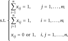
Denote the set of the failed SSs at the time t by K and the cardinality by
The first optimization (P1) precisely determines the minimum d, denoted by


Remark 2.
Under the condition that BSs can move at a constant velocity and the velocity of each BS is the same, the previous problem can be interpreted as the minimization of the recovery time which may improve the responsivity of the network to dynamic environments. Also, it is of great importance to reduce the maximum energy consumption of a single BS to prolong the lifetime of the network.
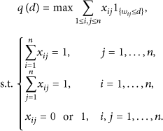
The second optimization (P2) is to find the optimal sensor scheduling strategy to minimize the total moving distances of BSs based on

In the previous two optimization problems, the first one involves the minimization of the energy of a single BS, while the second one is to minimize the total energy consumption of all BSs during the recovering process.
3. Optimal Sensor Scheduling
To maintain a guaranteed network coverage ratio, some spare BSs should be relocated to recover a necessary number of failed SSs. The optimal sensor scheduling problem will be studied according to the following steps. We will first investigate the relationship between the coverage ratio and the number of failed SSs, which can be readily used to determine the number of recovered sensors under different requirements of the coverage ratio
3.1. Coverage Ratio
The coverage ability measured by coverage ratio is one of the most important performances of WSNs. Specifically, the coverage ratio is defined as the ratio of covered area of active sensing SSs to the whole area of interest, that is,


The coverage ratio
3.2. Heading Scheduling Algorithm
Before proceeding further, we first provide the solution to optimization (P1).
Define
To get the optimal

The computation flow.
Concerning with the second optimization (P2), the authors in [10] transform the dispatch problem into maximum-matching problem and solve it by using a message passing algorithm [24]. Different from [10], the sensor dispatch problem in our work is a minimum matching problem. Further, the objective function in the optimization (P2) only deals with the distance that is less than
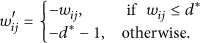
The rationale lies in the fact that if Initialization: At kth iteration: At kth iteration, we compute:


Estimation of
To the moment, the two optimization problems formulated in Section 2 can be solved, suggesting that our optimal sensor scheduling is feasible.
3.3. Discussion on Distributed Algorithm
Adopting the previous scheduling algorithm, we can get the optimal dispatch for BSs under the constraint that the minimum value of the largest moving distance is limited to
In the sequel, we define the neighbor BSs of uth BS by

In this setting, each BS receives information from SSs and simultaneously detects the number of failed SSs. It is sensible since energy expenditure in data processing or message reception is much less than that in transmission [1]. Once the number of failed SSs is greater than the critical number for a guaranteed coverage ratio, each BS will cooperatively implement the following distributed suboptimal scheduling. Specifically, at the initialization stage, a BS is firstly selected in a random fashion and will choose its closest failed SS as the initial matching. Next, another BS will be randomly chosen and the closest failed SS in the remaining SSs is considered as its matching. The same rule sequentially applies to the other BSs. Finally, each BS has a unique matching SS and vice versa. Then, they communicate the matching information with their neighbors and swap their matchings if the swapping will lead to a lower cost.
This process can be precisely formulated as follows. Let us focus on a specific uth BS. Assume that the uth BS is assigned to recover the

Remark 3.
The previous proposed initialization algorithm appears to require a centralized unit to notify the completion of the initialization for all the BSs since each BS only accesses neighbors' matching information. In practice, that is unnecessary because the swapping within two neighbor BSs can start regardless of other BSs' matching states, which means that there is no need to wait for all the BSs to obtain their initial matchings.
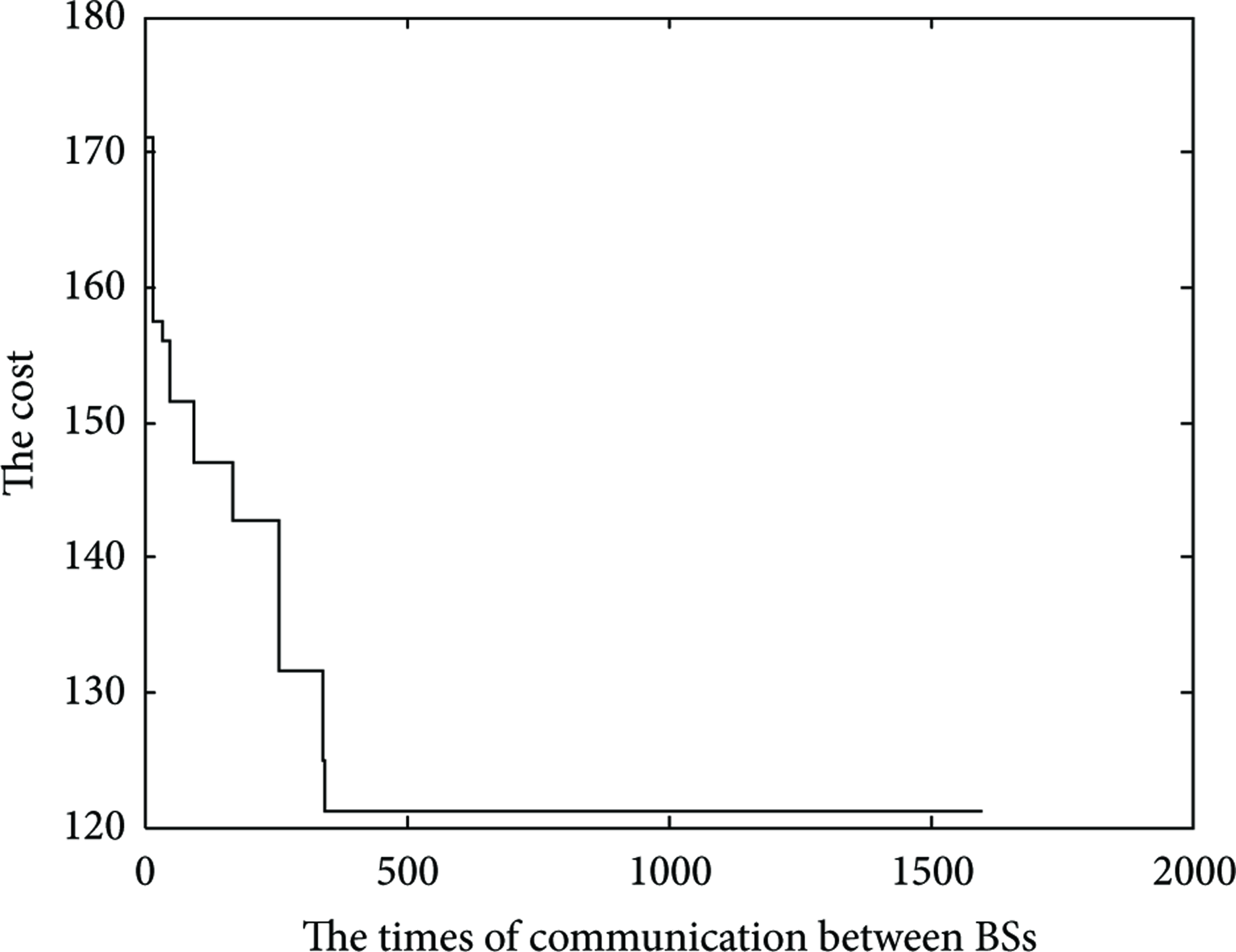
It is clear that each swap of the matching within two BSs will result in a lower cost, implying that the total cost is a decreasing function of the times of communication. Obviously, the total cost should be greater than zero, that is, lower bounded by zero. Thus, the total cost will converge to a limiting point after a sufficient large number of the communication times. Theoretically, although each communication may induce a lower cost, whether the limit is the minimum one among all possible matchings is unclear.
In the next section, some demonstrating examples would be examined to verify all the proposed algorithms on MATLAB 7.1 platform.
4. Simulations
4.1. Regular Network Topology
The sensing range of a sensor is set to

The regular network condition: failed sensors are denoted as “×”.
4.1.1. Centralized Optimal Scheduling
According to Figure 2, we can easily decide that how many failed sensors need to be recovered to guarantee the corresponding coverage ratio. Based on the optimization (P1), we get the relationship of
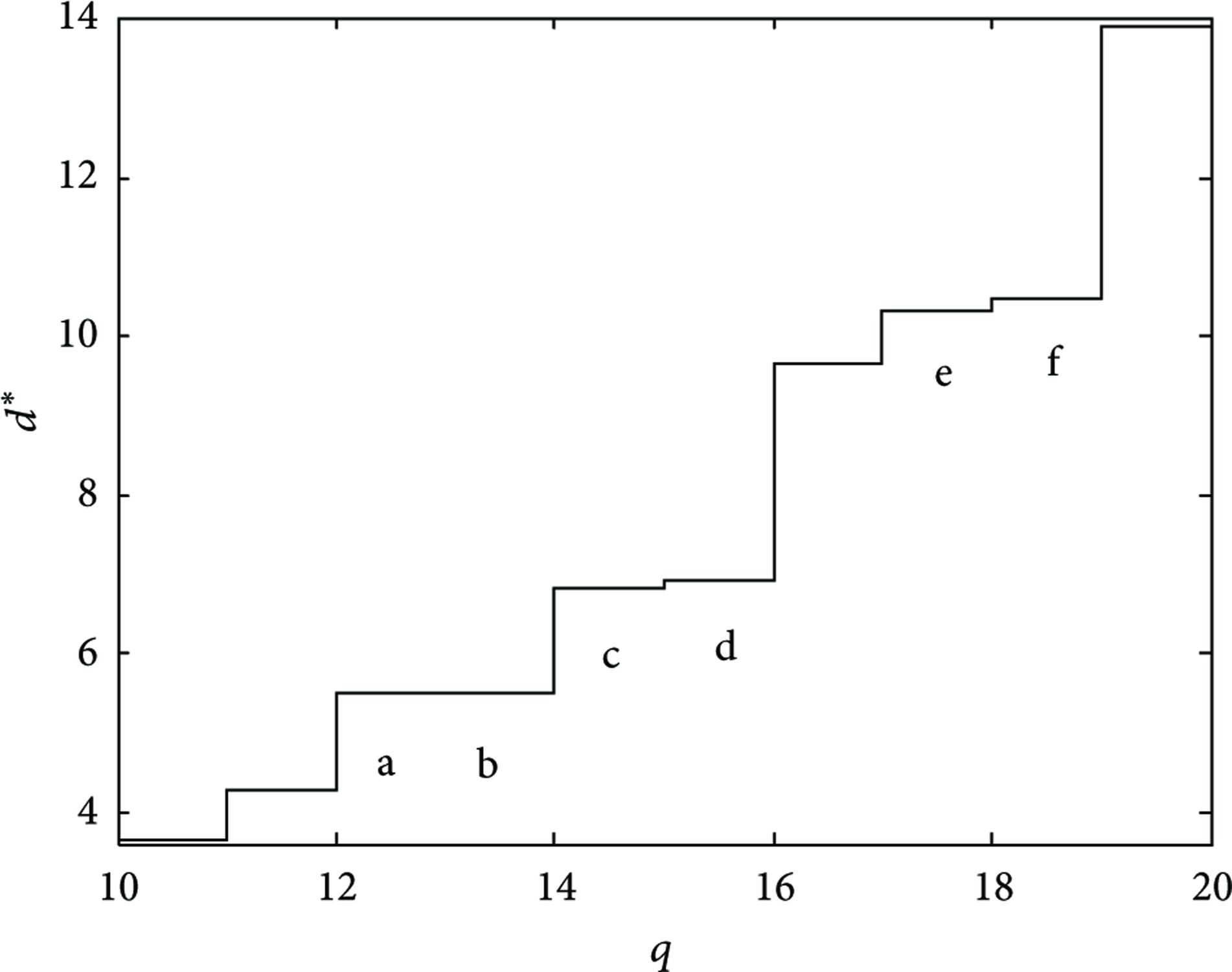
The number of failed sensors to be recovered q versus the minimum largest moving distance
Based on the optimization (P2), the optimal sensor scheduling result is obtained under a certain

The matching result to recover 10 failed sensors by the proposed centralized algorithm.
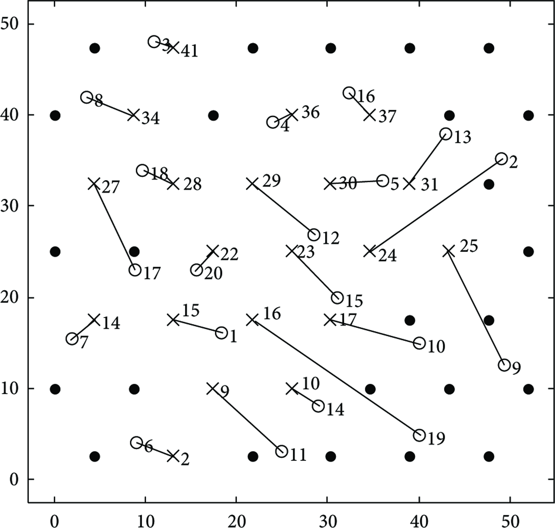
The more complicated case (20 recovered sensors) is illustrated in Figure 7. In this case, not every failed SS would be recovered by its closest BS. For instance, let us consider the matchings between the 10th SS and the 19th BS, the 16th SS and the 14th BS, and the 17th SS and the 15th BS. In Figure 7, the total cost of these dispatch matchings is

The matching result to recover 20 failed sensors by the proposed centralized algorithm.
The simulation results show that our algorithms can find an optimal solution for sensor scheduling. As indicated, the straight lines in Figures 6 and 7 are not the practical trajectory of moving BSs. If all activated BSs move along in a straight line, some of them would collide with working SSs and other moving BSs. For instance, in Figure 7, the 10th BS may collide with the 18th SS on its way to the location of the 24th failed SS. The 14th BS and the 19th BS may also collide with each other during the moving process. However, the focus of this paper is on the sensor dispatch, and path planning problem for moving sensors will be discussed in our future work.
4.1.2. Distributed Suboptimal Scheduling
According to the previous distributed suboptimal scheduling algorithm, the initial matching results of the case with 20 BSs and 20 SSs are illustrated in Figure 8. Here the initial matching randomly starts at the 14th BS, and it chooses the closest failed 10th SS as its initial matching. Proceeding with our distributed initialization algorithm, the next six BSs would obey the order of

The matching result by the proposed distributed initialization algorithm.
As mentioned previously, the connectivity of the communication topology is closely related to the value of R. Intuitively, the value of R is larger, the connectivity is better, which will lead to a better matching. However, R is obviously constrained by the available battery of BSs, while the near optimal matching can be achieved. Thus, the connectivity and the matching result under different values of R are discussed as follows.
Let R be
The comparison of the connectivity and the matching result under different values of R.
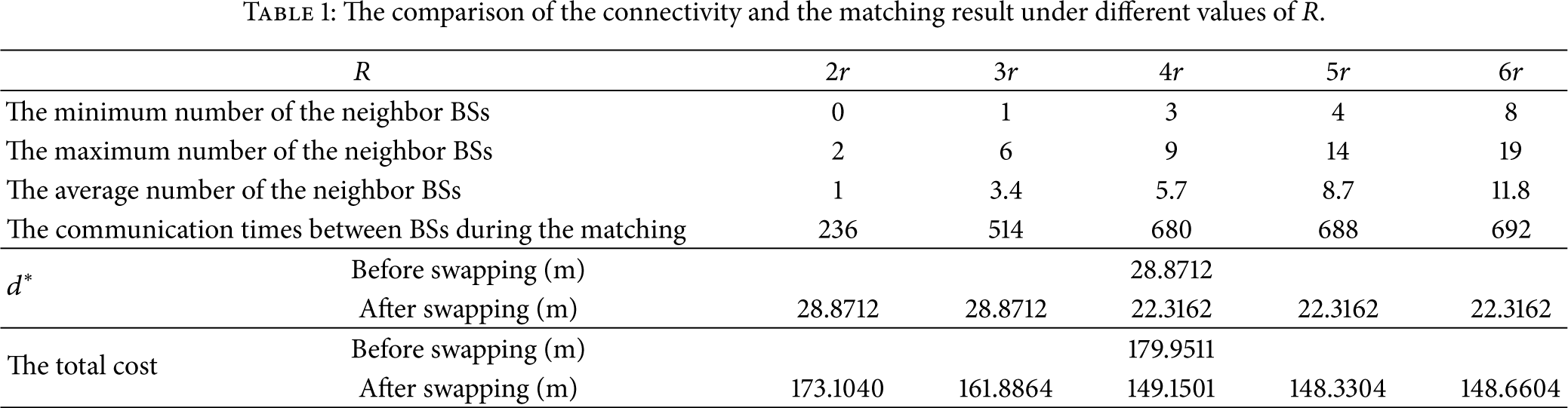
Setting

The communication topology of BSs for R = 20 m (4r).
The matching result to recover 20 failed sensors by the proposed distributed algorithm (

The matching result to recover 20 failed sensors by the optimal centralized algorithm (

The cost function with respect to the communication times.
4.2. Random Network Topology
As shown in Figure 13, the sensing range of a sensor is also set to
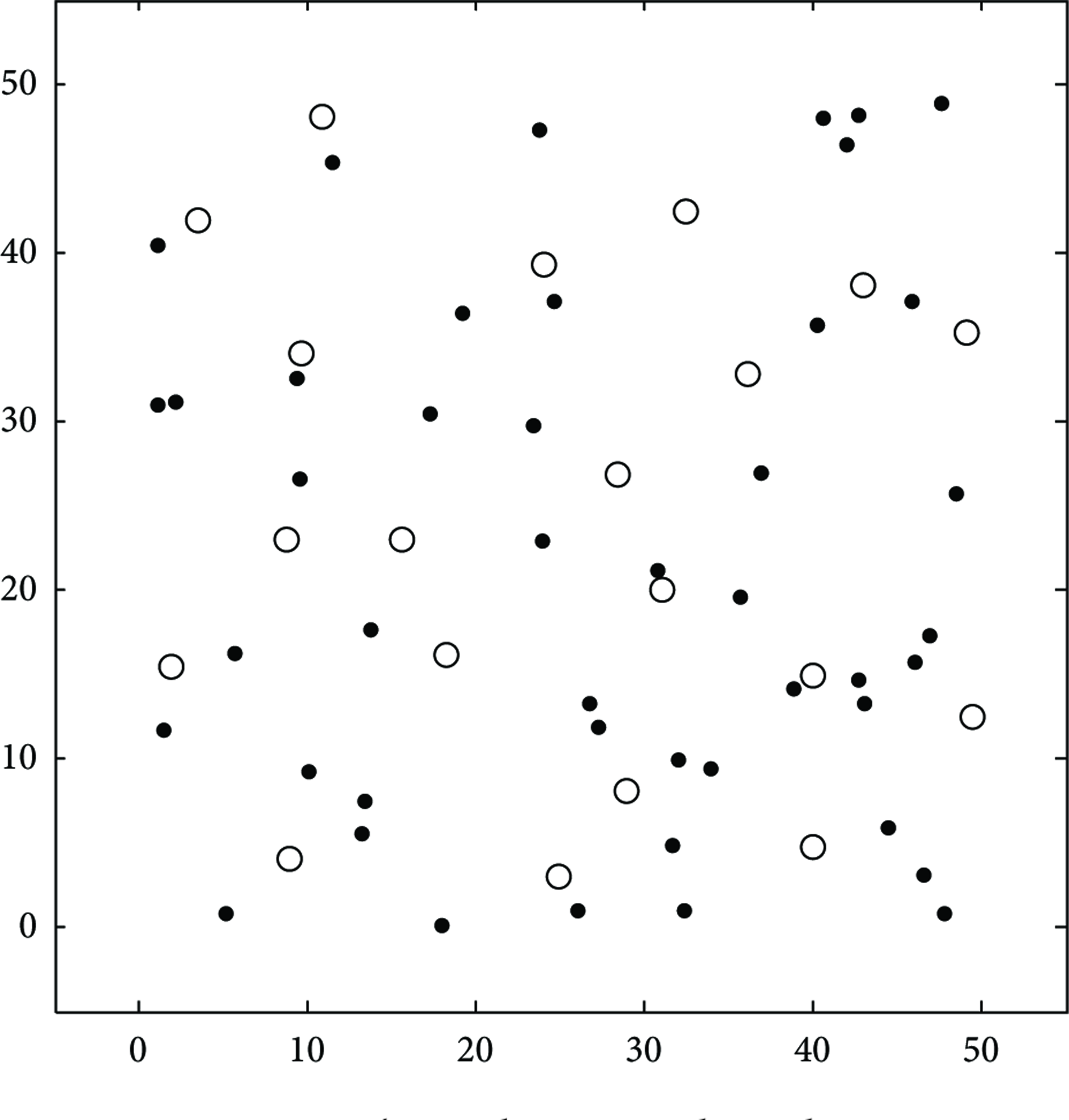
The random network condition.

Failed sensors are denoted as “×”.
4.2.1. Centralized Optimal Scheduling
The best performance that the centralized optimal scheduling can achieve under the limitation of maximum moving distance (see Figure 15(a)) is compared to that of the centralized optimal scheduling without the consideration of maximum moving distance (

The matching result to recover 20 failed sensors by the optimal centralized algorithm.
4.2.2. Distributed Suboptimal Scheduling
The initial matching results of the case with 20 BSs and 20 SSs are illustrated in Figure 16. Here the initial matching randomly starts at the 3th BS, and it chooses the closest failed 39th SS as its initial matching. It is clear that most of BSs have their closest failed SSs as the initial matchings. However, because the closest failed SSs of BSs

The initialization matching result.
Also setting

The final matching result.
The cost function with respect to the communication times.
5. Conclusions
We have proposed an optimal mobile sensor scheduling for WSNs with possible static sensor failures due to limited energy and other unknown factors. To maintain the coverage performance of the network, some spare mobile sensors should be deployed to recover failed sensors. Using a centralized FC, we formulated the sensor dispatch problem into two optimization problems and proposed two corresponding algorithms for their solutions. Our scheduling scheme first limited the maximum moving distance of the mobile sensors so as to reduce the maximum energy consumption of a single mobile sensor and then sought an optimal dispatch method to minimize the total moving distance. Removing the centralized FC, we also considered a distributed suboptimal sensor scheduling method which only depended on the local matching information of the neighbor mobile sensors. Simulation results verified the proposed algorithms under regular and random network topologies.
Footnotes
Acknowledgments
This work is supported by the National Science and Technology Support Program “study on the integration technology of large scale battery energy storage system” (no. 2011BAA07B07), the Natural Science Foundation of Jiangsu Province of China (no. BK2012409), and the Special Fund for Basic Scientific Research of Central Colleges, Hohai University (no. 2011B09014).