Sage Journals: Discover world-class research

Abstract

The aerodynamic characteristics of propeller-wing interaction for the rocket launched UAV have been investigated numerically by means of sliding mesh technology. The corresponding forces and moments have been collected for axial wing placements ranging from 0.056 to 0.5D and varied rotating speeds. The slipstream generated by the rotating propeller has little effects on the lift characteristics of the whole UAV. The drag can be seen to remain unchanged as the wing's location moves progressively closer to the propeller until 0.056D away from the propeller, where a nearly 20% increase occurred sharply. The propeller position has a negligible effect on the overall thrust and torque of the propeller. The efficiency affected by the installation angle of the propeller blade has also been analyzed. Based on the pressure cloud and streamlines, the vortices generated by propeller, propeller-wing interaction, and wing tip have also been captured and analyzed.

1. Introduction

Due to the high efficiency characteristics, the propeller is often used for the low-speed aircrafts, such as the straight-line aircrafts and short-range aircrafts. With the growth of the computing capability and update in the improvement of CFD methods, many researchers investigated the interference between propeller and fuselage numerically.

Strash and Lednicer [1] had conducted simulations to study the aerodynamic interferences between the propeller slipstream and fuselage. The corresponding results showed that the comparisons between computed and measured wing pressure data were good and the propeller thrust coefficient was within 12% of the experiment. Muller and Aschwanden [2] had conducted the wind tunnel tests to analyze the slip-flow effects of the rapid transit aircraft. During the tests they had developed a new type of engine system which can be successfully applied to the low-speed wind test. Boyle et al. [3] had investigated the aerodynamic characteristics of the propeller in the transonic and subsonic conditions, which was equipped with six blades. The flow field created by the propeller slipstream in the steady and unsteady flows had also been studied.

Gamble and Reeder [4] performed the static test and wind tunnel test, respectively, to study the interference characteristics between the propeller and wing. The results showed that between 12 and 18% of propeller thrust had been translated into airframe drag, with the largest percentage occurring for the wing placement closest to the propeller. In order to solve the unsteady flow problems of three-dimensional multichip blade in preflight condition, Boniface et al. [5] had simulated the waving and pitch movement of blades. One advantage of the dynamic grid was to be included in the actual blade waving and variable distance movement. Unfortunately, the drawback for this configuration is that the grid deformation will be happened at the middle of the region, which might affect the calculation results seriously. Meakin [6] had calculated the unsteady flow field and load of the oblique rotary-wing aircraft. However, the corresponding results had not been verified by any experiments. Whitfield and Srinivasan et al. [7, 8] had conducted simulations to calculate the hovering and the forward flight fields of a single rotor. The results showed that comparison of the numerical results at subsonic and transonic flow conditions was in good agreement with the experimental data for the surface pressures and the near field vortex trajectory.

With the previous considerations in mind, the effects of propeller placement with respect to the airframe on performance and aircraft handling on miniature air vehicles warrant are further considered. The study on the propeller design method has also little public available information. This paper will adopt the sliding mesh technology to investigate the unsteady aerodynamic characteristics of the propeller-wing interaction for the rocket launched UAV.

2. Flow Configurations and Computational Method

2.1. Rocket Launched UAV Configuration

As shown in Figure 1, the rocket launched UAV is initially folded into the narrow circular sleeve of the long-range missile. The folded components include the propeller, wing, and horizontal and vertical tails. This type of UAV can be released from the high altitude and coupled with a two-stage separated process, that is, the missile body flight at high angle of attack and UAV parachute packing tube; both of these make up the slow separation program. Carried by the deceleration parachute, the sleeve slowed down to the ground to a certain speed; the center of gravity of UAV will be hung by a line. The corresponding aerodynamic forces could enable UAV to maintain a balance. After breaking the parachutes, the UAV would start the cruise flight.

Figure 1:

Schematic view of the folding process for a rocket launched UAV.

The geometric parameters of the propeller model considered are listed in Table 1. The diameter of propeller is 271.65 mm and hub diameter is 28 mm. For the present study, we choose two blade type of propeller and the selected rotating speed ise 3000~10000 rpm. Clark-Y airfoil has been used for the blade. There are five factors for the pitch ratio and blade installation angle, respectively. The blade twist angle is chosen as 26.5°.

Table 1:

The parameters of the propeller considered.

Geometric parameters	Propeller

Propeller diameter/D	271.65 mm
Hub diameter/d₀	28.00 mm
Number of blades/N_B	2
Propeller rotational speed/n	3000 ~ 10000 rpm
Blade airfoil	Clark-Y
Blade width/b = f(r)	Max: 30.5 mm, Min: 9.92 mm
Blade thickness/C	Max: 4.312 mm
Pitch ratio	0.056D, 0.08D, 0.17D, 0.3D, 0.5D
Blade installation angle θ (r = 56%R)	30°, 38°, 45°, 50°, 55°
Blade twist angle/χ	26.5°

For the UAV, due to the fact that our present study mainly focuses on the interaction between the rotating propeller and wing, we have simplified the corresponding geometry into two parts: fuselage and wing, removing other component parts. The NACA0012 airfoil is used for wing. The corresponding span and chord of the wing are 1.2 m and 0.066 mm, respectively. The wingtip is totally straight rectangle without any forward or backward swept angles.

2.2. Computational Method and Governing Equations

2.2.1. Sliding Mesh Technology

As shown in Figure 2, the region of interface is composed of the surfaces A-B and B-C as well as the surfaces D-E and E-F, which can generate the surfaces a-d, d-b, and b-e, respectively [9, 10]. The two overlapped units can create the surfaces d-b, b-e, and e-c, which will form the inner airflow area. The surfaces a-d and c-f will form the periodic region. During calculating the airflow of the unit IV, we can use the surfaces d-b and b-e instead of the surfaces D-E, and the corresponding information will be transmitted to the unit IV via the units I and III.

Figure 2:

The schematic diagram for the sliding mesh technology.

In the sliding mesh calculation, computational domain mainly contains two relative movements of the subdomains. Each domain has at least one interface whose subdomain is connected to the adjacent subdomains. The entire grid computing regions are divided into two parts: inner and outer flow fields. The inner field encloses the surfaces of propeller, and the outer field is the outermost layer of the entire region which will be made as the velocity inlet and pressure outlet boundary conditions. The junction of the middle channel will be set as “interface.” Sliding mesh is often used for the nonstructure grids. The inner and outer flow fields will exchange fluxes through the interpolation. Both sides of the subdomain at the junction of the surface will not share the same grid nodes and maintain the flux conservation. The amount of relocation within the boundaries of the region will be calculated based on the relative movement between the subdomains.

2.2.2. Governing Equations

The sliding mesh model is a special case of general dynamic mesh motion wherein the nodes move rigidly in a given dynamic mesh zone. Additionally, multiple cells zones are connected with each other through nonconformal interfaces. As the mesh motion is updated in time, the nonconformal interfaces are likewise updated to reflect the new positions for each zone.

It is important to note that the mesh motion must be prescribed such that zones linked through nonconformal interfaces remain in contact with each other (i.e., “slide” along the interface boundary) if the fluid is able to flow from one mesh to the other. The integral form for any flow scalar φ in any control body's transport equation can be written as

\frac{d}{d t} \int_{V} ρ φ d V + \int_{\partial V} ρ φ (\overset{⇀}{u} - {\overset{⇀}{u}}_{g}) \cdot d \overset{⇀}{A} = \int_{\partial V} Γ \nabla φ \cdot d \overset{⇀}{A} + \int_{V} S_{φ} d V,

(1)

where ρ is the gas density, $\overset{⃑}{u}$ is the uniform flow velocity, ${\overset{⃑}{u}}_{g}$ is the sliding mesh speed, Γ is the dissipation factor, S_φ is the source term, and dV stands for control volume boundary.

The fundamental difference between sliding mesh transport equation and ordinary transport equation lies in the representative grid movement,

- \int_{\partial V} ρ φ {\overset{⇀}{u}}_{g} \cdot d \overset{⇀}{A} .

(2)

Because the mesh motion in the sliding mesh formulation is rigid, all cells retain their original shape and volume. As a result, the time rate of change of the cell volume is zero. So the control volume V^{n + 1} at any n + 1 moment can be calculated as

V^{n + 1} = V^{n} .

(3)

Then the first-order backward difference discrete will be simplified to

\frac{d}{d t} \int_{V} ρ φ d V = \frac{[{(ρ φ)}^{n + 1} - {(ρ φ)}^{n}] V}{Δ t},

(4)

where n and n + 1 represent the current time and the subsequent moment, respectively.

2.2.3. Boundary Conditions

As shown in Figure 3(a), in the stationary zone of the UAV, the calculation domain was divided into 24 subdomains, which would be meshed with structural grids. During meshing the unstructured grids in the dynamic zone for the propeller, as shown in Figure 3(b), the size function has been adopted to control grid size and generate the five-layer 1.3 times the scale of three prism grids near the blade surfaces [13]. The stationary zone and dynamic zone are combined with interface technology, generating all the computational flow of the rocket launched UAV propeller.

Figure 3:

Decomposition of the computational domain.

The radial length of the computational domain is 30 times of the cross-section the UAV fuselage. The whole mesh has been smoothed and swapped, which can rebuild the nodes, modify the connectivity of units, and improve the accuracy of the calculation. The free stream velocity considered is at 25 m/s and the corresponding Reynolds number (Re) is based on 1.6 × 10⁵. In the numerical simulation, the couple-implicit solver is used. SIMPLE iteration is adopted with the wall functions.

2.3. Theoretical Calculation for the Thrust Force Created by the Rotating Propeller

As shown in Figure 4, φ₀ represents the angle between the synthesis speed and rotation plane.

Figure 4:

Corrected blade element theory (angles and velocity relationship) [12 –14].

Consider

φ_{0} = arc t g \frac{V}{π \cdot d \cdot n},

(5)

where V is the UAV flight speed and n is the rotating speed of the propeller. Then the lift force created by the rotating propeller can be written as

C_{L} = \frac{0.1 d}{d + 1.82 c} [\frac{180 ∊}{π} (arc t g \frac{e}{π \cdot d} - arc t g \frac{V}{π \cdot d \cdot n}) - α_{0}],

(6)

where e is the geometric pitch, d is the diameter of propeller, ε represents the downwash corrected factor (ε = 0.95), α₀ is the zero lift angle of attack for propeller blade (α₀ = – 5°), j is the chord exhibition position reference (j = 0.5), and i is the blade utility area coefficient (i = 0.8). According to the lift equation, the corresponding force can be written as

\begin{matrix} L = \frac{ρ \cdot c \cdot i \cdot d^{2}}{20 d + 36.4 c} [V^{2} + {(π \cdot j \cdot d \cdot n)}^{2}] \cdot [\frac{180 ∊}{π} (arc t g \frac{e}{π \cdot d} - arc t g \frac{V}{π \cdot d \cdot n}) - α_{0}], \\ γ = arc t g (C_{D_{f}} + \frac{k_{i} \cdot c}{π} \cdot \frac{0.01 d}{{(d + 1.82 c)}^{2}} \times {[\frac{180 ∊}{π} (arc t g \frac{e}{π \cdot d} - arc t g \frac{V}{π \cdot d \cdot n}) - α_{0}]}^{2}) \times (\frac{0.1 d}{d + 1.82 c} [\frac{180 ∊}{π} (arc t g \frac{e}{π \cdot d} - arc t g \frac{V}{π \cdot d \cdot n}) {- α_{0}])}^{- 1}, \end{matrix}

(7)

where γ represents the drag-lift angle, and k_i is the corrected factor for the blade tip shape (k_i = 1.30). Then the thrust force created by the rotating propeller can be written as

T = \frac{L \cdot \cos (φ_{0} + γ)}{\cos γ} .

(8)

3. Results and Discussion

3.1. Comparison of the CFD, Theoretical, and Experimental Results

Firstly we should test the grid sensitivity; we have chosen six different grid sizes (A × B, y) to simulate the whole propeller-wing configuration (A: nodes on the perimeter edges of the outer computational domain, B: nodes in the axial direction, y: the minimum grid spacing on the propeller blades). c is the chord length of the wing. They are 201 × 201, 3e – 5c; 401 × 201, 3e – 5c; 201 × 101, 2e – 5c; 201 × 101, 5e – 5c; 201 × 101, 0.5e – 5c; and 201 × 101, 3e – 5c, respectively. From Figure 5 we can see that the six grid sizes studied do not deviate from each other within 2%. As a result, we adopt the 401 × 201, 3e – 5c grid for the subsequent computation.

Figure 5:

Grid sensitivity test.

Subsequently, the reliability of the numerical method should be verified. The test model now is the same as the experimental test [11]. The thrust characteristics of the rotating propeller at different rotating speeds are compared.

As shown in Table 2, the theoretical data has shown the excellent agreement with the experimental data, showing that this theory can be used to predict the thrust force generated by the rotating propeller. For the CFD data, the maximum difference is within 4.53% comparing with the experimental data from Chen et al. [11], and the minimum difference is within 0.5%. Considering the accuracy of the measurement method and the simulation errors, the comparisons are showing reasonable overall quantitative agreement, showing the accuracy of the present CFD approach.

Table 2:

The comparison of experimental, theoretical, and CFD data (propeller only).

Rotating speed (rpm)	1948	3600	4410	5430	6360	7110	7620

Experiment*	0.223	0.752	1.078	1.666	2.352	2.940	3.528
Theory	0.2198	0.7508	1.1267	1.7082	2.3434	2.9287	3.3639
Error (%)	1.43	0.16	4.52	2.53	0.37	0.38	4.65
CFD	0.2331	0.7625	1.1263	1.6758	2.3622	2.9519	3.4519
Error (%)	4.53	1.40	4.48	0.59	0.43	4.05	2.16

Chen et al. [11].

Figure 6 has shown that the thrust, torque, and propeller efficiency changed with different rotating speeds for the present studied propeller model. From the previous figures we can see that the thrust force and torque are increasing with the increase of the rotating speed (ranging from 3000 to 10000 rpm). For the propeller efficiency, the corresponding curve has experienced firstly an increasing and then a decreasing trend. The efficiency will reach the maximum at about n = 6000 rpm in values. Therefore, we choose n = 6000 rpm for the subsequent computation.

Figure 6:

The thrust, torque, and propeller efficiency versus different rotating speeds (V = 25 m/s).

3.2. Propeller-Wing Interaction (without Flight Speed)

As shown in Table 3, a representative portion of a data set for the speed setting of 6000 rpm and fixed Z₀ = 0 is included to show the various forces and moments. The lift created by the propeller is almost zero for the present studied propeller locations. The drag can be seen to remain relatively unchanged as the wing moved progressively closer to the propeller until 0.056D away from the propeller, where a nearly 20% increase occurred. However, the varied propeller position X₀ has a negligible effect on propeller thrust and torque.

Table 3:

Forces and moments for n = 6000 rpm, V = 0.

X₀/D	Z₀/D	Lift, N	Drag, N	Roll moment	Thrust	Propeller torque

0.056	0	0.0009 ± 0.002	2.043 ± 0.04	0.0030 ± 0.001	10.84 ± 0.03	0.4996 ± 0.01
0.08	0	0.0014 ± 0.002	0.085 ± 0.04	0.0042 ± 0.001	10.83 ± 0.03	0.4982 ± 0.01
0.17	0	0.0012 ± 0.002	0.077 ± 0.04	0.0027 ± 0.001	10.78 ± 0.03	0.4979 ± 0.01
0.3	0	0.0011 ± 0.002	0.080 ± 0.04	0.0029 ± 0.001	10.83 ± 0.03	0.4876 ± 0.01
0.5	0	0.0010 ± 0.002	0.089 ± 0.04	0.0017 ± 0.001	10.80 ± 0.03	0.4872 ± 0.01

The reason for the almost zero lift can be mainly attributed to the effect of the rotating propeller shown in Figure 7; the entire aircraft will be subjected to the slip flow region created by the rotating propeller. As the blades rotate counterclockwise, this can produce the upwash effect on the right wing and downwash on the left wing. Consequently, the effective angles of attack of the right wing will be increased and the corresponding lift will be increased. Affected by the downwash effect, the effective angles of attack for the left wing will be decreased, and then the lift will be decreased. These two effects compensate each other, making the lift have no significant change.

Figure 7:

The 3D streamlines for the rotating propeller domain.

The axial induced velocity created by the rotating propeller can generate induced resistance. When the propeller moves closer to the wing, the corresponding impacts on the entire aircraft will become greater, so the resistance can reach the maximum at the close-coupled position. Because the rotating propeller could generate thrust by itself and it is also affected by the reaction force from the aircraft, these effects are quite small. Therefore the basic thrust always remains unchanged. Without the air flow, the torque of the propeller has not been affected by the flow, which was only created by the rotating motion, so the torque has also remained constant.

For a constant flying speed, if the rotating speed increases, the blade tangential velocity will be increased and the corresponding pitch ratio ( $λ = V / n D$ ) will be decreased. The propeller thrust and torque are always increasing as the speed increases within a certain range. However, the efficiency of the propeller is not always proportional to the rotating speed. The tip speed of the blades $W_{R} = \sqrt{V^{2} + {(π D n)}^{2}}$ , and the tip Mach number $M_{a R} = W_{R} / C = \sqrt{V^{2} + {(π D n)}^{2}} / C$ . M_aR is directly related to the flight speed, propeller diameter, and rotating speed. If the rotating speed is too fast, M_aR can reach the higher value, due to the effects of air compression. This can create shockwave loss on the paddle tip and result in a sharp decline in the efficiency of the propeller. It even can produce a great aeroacoustic. In order to make the efficiency of the propeller reach the maximum level in flight state, M_aR should be maintained not more than 0.95~0.97. By reducing the circumference tip speeds of the propeller to reduce M_aR can become feasible.

3.3. Propeller-Wing Interaction (with Flight Speed)

As shown in Table 4, the lifts on the right and left wing have been changed due to the propeller slipstream effect. However, in the slip flow region, the right and left wings have experienced the induced resistance, so drag characteristics remained basically unchanged. Based on this, we intercepted four sections, which are located at z = 0.05, −0.281, −0.65, and 0.03, which are relative to the head of aircraft (z = 0).

Table 4:

Forces for n = 6000 rpm, V₀ = 25 m/s.

X₀/D	Z₀/D	Lift, N (left)	Drag, N (left)	Lift, N (right)	Drag, N (right)

0.056	0	− 0.972 ± 0.2	0.71 ± 0.003	0.972 ± 0.2	0.71 ± 0.003
0.08	0	− 0.910 ± 0.2	0.71 ± 0.003	0.910 ± 0.2	0.71 ± 0.003
0.17	0	− 1.020 ± 0.2	0.71 ± 0.003	1.020 ± 0.2	0.71 ± 0.003
0.3	0	− 1.021 ± 0.2	0.71 ± 0.003	1.021 ± 0.2	0.71 ± 0.003
0.5	0	− 1.025 ± 0.2	0.71 ± 0.003	1.025 ± 0.2	0.71 ± 0.003

In section I (z = 0.05 m) shown in Figure 8(a), the rotating propeller has generated the vortices, which have the same direction as the rotating propeller. The vortex core is at the center of vortex, and its intensity is also the largest. The convolution effect in the middle of the blade has reached the maximum. However, due to the propeller tip effect, both ends of the wing tip have generated other two secondary vortices at the same time. Two vortices have been shown to be anti-symmetric with the axis.

Figure 8:

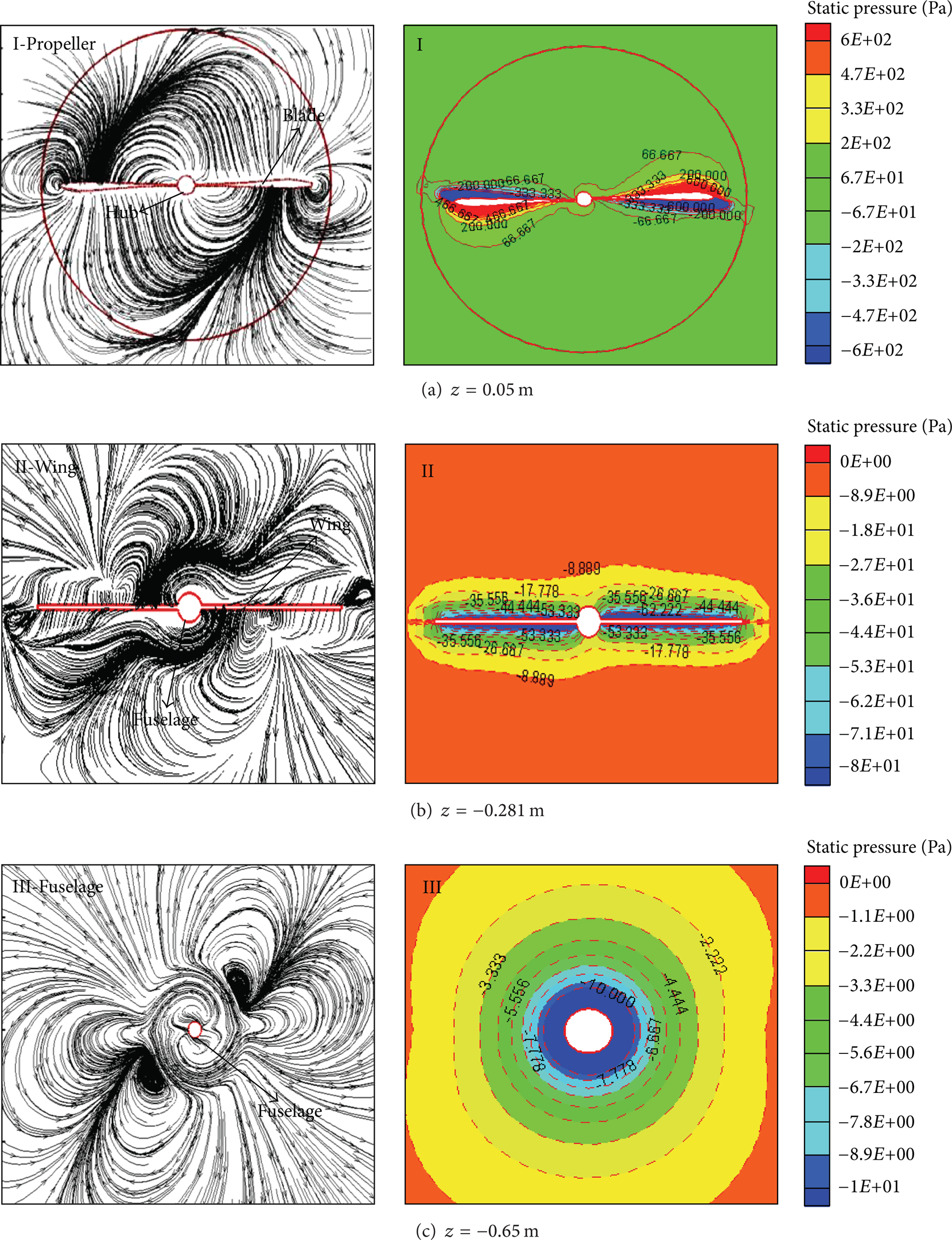
Different sections of the vortex structure.

When the air flows over section II (z = – 0.281 m) shown in Figure 8(b), the flow pattern is roughly the same as in section I. The only difference is that the vortex intensity has been reduced. The closer to the wing root, the faster the air will be accelerated. Both the bottom of the left wing tip and the top of the right wing tip have generated their own vortices. The corresponding pressure cloud has also shown that, due to the propeller slipstream effect, the wing surface pressure distributions have shown apparent asymmetry.

When the flow developed closer to horizontal tail, that is, section III (z = – 0.65 m) shown in Figure 8(c), both the lower left side and the upper right side of the fuselage have generated a clear vortex core. And the flow around the vortex core has shown two opposite directions.

But between the propeller and wing shown in Figure 9, the slipstream generated by the rotating propeller has been roughly divided into three parts. (1) The inner layer has created a whirlpool, where the core is in the center. The rotating direction of the airflow around the propeller has been shown to be the same as the direction of the rotating propeller. (2) The outer layer: the airflow has been speeded up along the axis and caused the vortices. (3) The middle layer: two “ears” have been generated here, and the vortex core is not clear. All of these fully showed that the slipstream of the propeller is constantly changing along the axial direction.

Figure 9:

The streamlines in section IV (z = 0.03 m).

As shown in Figure 10, whether the propeller is on or off, the static pressure distributions around the upper and lower left and right wing surfaces have been changed. Firstly, the lower surface of the left wing along the spanwise has changed in trend. To take the left wing for example, without the propeller, the static pressure distributions along the spanwise are gradually reduced in the direction to the wing root (absolute). However, when the propeller begins to rotate, the overall trend of the static pressure distributions is showing the negative increase trend. Then the upper surface is shown to be different from the lower surface. Comparing with the no propeller case, the overall trend of the static pressure distributions for the propeller on case is almost identical, but it has about 12% of the negative directional increase.

Figure 10:

Comparison of the static pressure on the upper and lower surfaces of the left and right wings.

In the theoretical calculation, the slipstream diameter should remain unchanged. However, the propeller slipstream will be mixed with the surrounding air and the viscous dissipation; this can make the slipstream diameter diffuse outward continuously. As shown in Figure 11, the effects on the left and right wings created by the propeller slipstream are basically concentrated near the fuselage, and the spanwise scale is always located between 0 and 0.03 m; after that, the propeller slipstream effect on the wing will get much weaker.

Figure 11:

The front view of the particle trajectory flowing over the propeller wing.

The angle between the profile chord line and rotating propeller surface is defined as blade installation angle θ. In order to make the entire propeller blade work under the favorable angle of attack, the blades must be reversed in the radial direction. Therefore, the blade installation angle θ will be always changed along the blade radius direction. In the present study, we mainly select four typical installation angles for the further research: θ = 30°, 38°, 45°, 50°, 55°. The blade twist angle χ is set as 26.5°.

As shown in Table 5, keeping V and n unchanged, as the blade installation angle θ increases, the thrust will be constantly increasing. The effective power of the propeller is also increasing at the same time. However, for the torque of the propeller blades, because the installation angle increases, it has made the effective angle of attack increased when the air flowed through the blade. So both the torque relative to the propeller hub and the absorbed power P_w are increasing.

Table 5:

Comparison of the results for N = 6000 rpm, V = 25 m/s.

X₀/D	Z₀/D	T	M	P _w	P _e	η

30°	0	3.11 ± 0.03	0.2687 ± 0.01	168.82421	77.75	46.05%
38°	0	10.90 ± 0.03	0.6237 ± 0.01	391.87071	272.5	69.54%
45°	0	11.84 ± 0.03	1.0103 ± 0.01	634.77149	296.0	46.63%
50°	0	13.18 ± 0.03	1.2822 ± 0.01	805.60626	329.5	40.90%
55°	0	13.64 ± 0.03	1.5726 ± 0.01	988.06458	341.0	34.51%

However, the efficiency of the propeller is not always proportional to the size of blade installation angle θ. As shown in Figure 12, the efficiency of propeller η has reached to maximum at θ = 38°. In other positions, η cannot achieve its best. This is mainly due to the fact that the air flowing through each section of the blade is composed of the forging speed along the rotating axis and the tangential speed created by the rotation. When the installation angle (θ) increases to a certain value, angle of attack of the blade will reach its greatest. However, in some profiles, the angle of attack is too large which can exceed the stall boundary. Once happened, the aerodynamic characteristics of the propeller would become bad. The thrust created by the propeller will also decrease sharply. The thrust curve has also tended to be moderate at θ = 50° and 55°.

Figure 12:

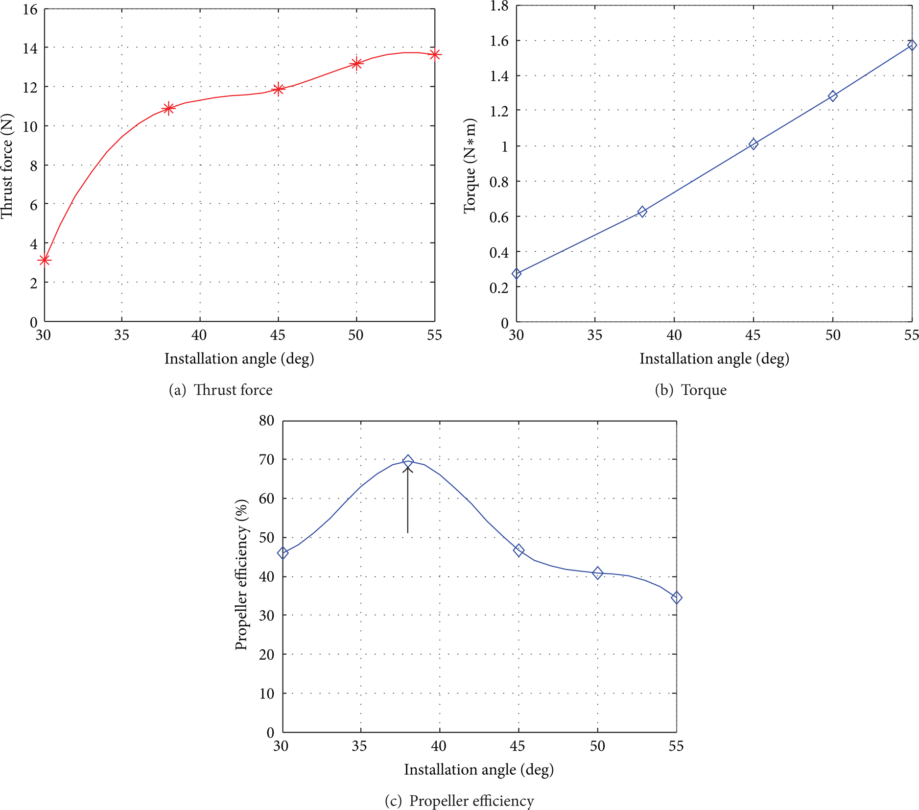
The thrust, torque, and efficiency versus different installation angles (at 60% D).

4. Conclusions

As the propeller rotates counterclockwise, it can produce the upwash effect on the right wing and downwash on the left wing. These two effects compensate each other, making the slipstream generated by the rotating propeller have little effect on the lift characteristics of the whole rocket launched UAV.

The axial induced velocity created by the rotating propeller can generate induced resistance. As the propeller moves closer to the wing, the impacts on the entire aircraft will become greater. The corresponding drag can reach its maximum at the close-coupled position (about 20% increment).

Because the rotating propeller can generate thrust by itself and it is also affected by the reaction force from the aircraft, these effects were quite small, and the basic thrust remains constant. When there is no flight speed, the torque of the propeller will not be affected by the airflow it is only generated by the rotating motion. So the torque always remains unchanged and has nothing to do with the varied pitch ratio.

Comparing with the absence of the propeller, in the presence of the propeller slipstream, the lower surface of the wing along the spanwise has changed in trend, but the upper surface is different from the lower surface. The overall trend of the static pressure distribution is identical, but it has about 12% of the negative directional increase.

Footnotes

Nomenclature

Acknowledgments

Deepest gratitude goes first and foremost to Professor Yu, Professor Chien, and Professor Xu for their constant guidance. Financial support from Nanyang Technological University is gratefully acknowledged. The authors also would like to thank the reviewers for their helpful suggestions.

References

Strash

D. J.

and Lednicer

D. A.

, “Analysis of propeller-induced aerodynamic effects,” in Proceedings of the 16th AIAA Applied Aerodynamics Conference, AIAA-1998-2414, 1998.

Muller

and Aschwanden

, “Wind tunnel simulation of propeller effects in the A400M FLA-4 model,” in Proceedings of the 41st AIAA/ASME/SAE/ASEE JJoint Propulsion Conference & Exhibit, July 2005.

Boyle

F. J.

Flaherty

M. P. O.

, and Eaton

J. A.

, “Validation of efficient euler algorithms for advanced propellers under transonic and subsonic conditions,” in Proceedings of the 17th Applied Aerodynamics Conference, June-July 1999.

Gamble

B. J.

and Reeder

M. F.

, “Experimental analysis of propeller-wing interactions for a micro air vehicle,” Journal of Aircraft, vol. 46, no. 1, pp. 65–73, 2009.

Boniface

J. C.

Mialon

, and Sides

, “Numerical simulation of unsteady euler flow around multibladed rotor in forward flight using a moving grid approach,” in Proceedings of the 51st Annual Forum of AHS, pp. 821–834, May 1995.

Meakin

R. L.

, “Moving body overser grid methods for complete aircraft tiltror simulation,” in Proceedings of the 11th Computational Fluid Dynamics Conference, AIAA-1993-3350-CP, 1993.

Whitfield

D. L.

, “Three-dimensional euler equations simulation of propeller-wing interaction in transonic flow,” in Proceedings of the AIAA 21stAerospace ScienceMeeting, 1983.

Srinivasan

G. R.

Baeder

J. D.

Obayashi

, and Mccroskey

W. J.

, “Flowfield of a lifting rotor in hover: a Navier-Stokes simulation,” AIAA Journal, vol. 30, no. 10, pp. 2371–2378, 1992.

Moffitt

B. A.

Bradley

T. H.

Parekh

D. E.

, and Mavris

, “Validation of vortex propeller theory for UAV design with uncertainty analysis,” in Proceedings of the 46th AIAA Aerospace Sciences Meeting and Exhibit, January 2008.

10.

Zhang

G. Q.

and Yu

S. C. M.

, “Unsteady aerodynamics of a morphing tandem wing unmanned aerial vehicle,” Journal of Aircraft, vol. 49, no. 5, pp. 1315–1323, 2012.

11.

Chen

Yang

S. X.

, and Mo

, “Modeling and experimental analysis of UAV electric propulsion system,” Journal of Aerospace Power, vol. 24, no. 6, pp. 1339–1344, 2009.

12.

Filippone

and Mohamed-Kassim

, “Multi-disciplinary simulation of propeller-turboprop aircraft flight,” Aeronautical Journal, vol. 116, no. 1184, pp. 985–1014, 2012.

13.

Verma

Jang

, and Mahesh

, “The effect of an upstream hull on a propeller in reverse rotation,” Journal of Fluid Mechanics, vol. 704, pp. 61–88, 2012.

14.

Whitmore

S. A.

and Merrill

R. S.

, “Nonlinear large angle solutions of the blade element momentum theory propeller equations,” Journal of Aircraft, vol. 49, no. 4, pp. 1126–1134, 2012.