Sage Journals: Discover world-class research

Abstract

The shaft tubular turbine is a form of tidal power station which can provide bidirectional power. Efficiency is an important turbine performance indicator. To study the influence of runner design parameters on efficiency, a complete 3D flow-channel model of a shaft tubular turbine was developed, which contains the turbine runner, guide vanes, and flow passage and was integrated with hybrid grids calculated by steady-state calculation methods. Three aspects of the core component (turbine runner) were optimized by numerical simulation. All the results were then verified by experiments. It was shown that curved-edge blades are much better than straight-edge blades; the optimal blade twist angle is 7°, and the optimal distance between the runner and the blades is 0.75–1.25 times the diameter of the runner. Moreover, the numerical simulation results matched the experimental data very well, which also verified the correctness of the optimal results.

1. Introduction

Tidal power generated by falling and rising water, which is a kind of potential energy [1], can transform mechanical energy into electricity. More specifically, a dam is built to back up the water located adjacent to bays or estuaries which are separate from the ocean and therefore form a reservoir. A hydroelectric generating set is then installed in the dam, and the pressure of the water from all tidal states turns the wheel, a motion which can be used to make electric power. The tubular turbine is applicable to tidal power stations because it can provide power from low water levels. The tubular turbine offers good technical and economic feasibility, which has contributed to its wide use and rapid development since its advent in the 1930s. In hydropower developments below 25 m level power, the tubular turbine has largely displaced the axial turbine, and therefore it is typically used for tidal power. Currently, the largest per unit installed capacity is 65.8 MW (bulb turbine in Japan only), the largest runner diameter has reached 8.2 m (shaft-well tubular turbine in America), and the highest power level is 22.45 m (bulb turbine in Japan) [2 –4]. Since the 1960s, research and application of tubular turbines has been well developed in China, and the largest runner diameter of an operating bulb tubular turbine is now 7.5 m. Tubular-turbine hydropower stations have been planned and constructed all over the country. The hydropower station constructed in Changzhou Guangxi includes 15 turbine installations and 621.3 MW installed capacity [5].

Shaft-extension type tubular turbines and shaft tubular turbines have almost the same advantages of technical and economic feasibility as bulb tubular turbines for low-water-level power stations. However, shaft tubular turbines have been used only in a few stations with relatively low capacity in China. The main reason for this is that the key technologies of flow-passage design, integrated turbine structure, corrosion-resistant blades, methods of connecting the speed-increase gearbox, and arrangement of the oil head in a double adjustable structure are still unsupported by thorough research and design, with the result that the shaft tubular turbine is still undeveloped and underutilized, although it offers simple structure and good performance, is easy to install and maintain, and is from 20% to 60% cheaper than the bulb tubular turbine. Therefore, research into these new types of tubular turbines is a far-reaching, significant, and urgent task so that the costs of construction and operation can be reduced and the development of this turbine in tidal power plants can be promoted.

2. Working Principles

Figure 1 shows a profile view of a shaft tubular turbine in a tidal power plant. The 2D flow channel in the bidirectional shaft tubular turbine includes five parts: the inlet section, the shaft section, the guide-vane section, the wheels, and the draft tube section. The generator and the speed-change unit as described above are arranged on the shaft. The movable guide vane described above is arranged in the guide-vane section, which is installed before the inlet in the side of the turbine wheel. The principal axis described above is connected to the water turbine, speed-increase unit, and generator, which transmits the mechanical energy from the water turbine into the speed-increase unit and the generator. The water turbine described above is set in the runner chamber of the runner section. The runner described above is arranged at the end of the principal axis of the water turbine.

Figure 1:

2D view of the flow channel in a bidirectional shaft tubular turbine; (b) is the top view of (a). 1 indicates the inlet section, 2 is the shaft section, 3 is the guide-vane section, 4 is the movable guide-vane section, 5 is the draft tube section, 6 is the principal axis, 7 is the movable guide vane, 8 is the wheels, 9 is the generator, and 10 is the speed-change gearbox.

Working Principle [6, 7]. The turbine is installed as part of the bidirectional tidal power plant. After the tide starts to rise, the gate is closed when the tidal water level and the water level in the plant are close to equal. As the tide level continues to rise, a situation with internal low and external high water levels is created. The water turbine goes into operation and starts to generate electricity when the water head is higher than the minimum allowable working head. At the same time, water from the open ocean flows into the reservoir, raising the water level in the reservoir. The tide continues to rise rapidly, as well as the working head level, until high tide. When the tide starts to fall, the water level in the reservoir becomes high. The water turbine is shut down when the water head is lower than the minimum allowable working head. The main advantage of this type of tidal power plant is that it can generate electricity during both rising and falling tides except when the water levels in the internal and external reservoirs are equal. Therefore, the generation operating time and generation capacity are greater than those of a one-way tidal power station, making full use of tidal energy. The flow is in opposite directions at different times, and the turbine operates bidirectionally. In addition, the turbine has good energy conversion performance in both operating modes. Consequently, this turbine can extract as much tidal energy as possible, improve energy usage, and increase the benefits of tidal power.

3. Numerical Simulation [8 –12]

3.1. Basic Equations

The continuity equations (incompressible viscous flow continuity equations) are

\frac{\partial u_{i}}{\partial x_{i}} = 0,

(1)

where u_i represents the instantaneous velocity in flow direction I and x_i represents the coordinates.

The Reynolds average model, which is widely applied in engineering, was used in this research. The Reynolds-averaged Navier model is obtained through the Navier-Stokes equations, which were averaged with the Reynolds-averaged equations. Averaged turbulence equations will contain pulsating second-order correlation measurements. For the closed equation, the corresponding equation turbulence model was introduced.

For the N-S Reynolds-averaged equations, it is possible to state that

\frac{\partial (u_{i})}{\partial t} + (u_{j}) \frac{\partial (u_{i})}{\partial x_{j}} = - \frac{1}{ρ} \frac{\partial (p)}{\partial x_{i}} + υ \frac{\partial^{2} (u_{i})}{\partial x_{j} \partial x_{j}} - \frac{\partial (u_{i}^{'} u_{j}^{'})}{\partial x_{j}} + 〈 f_{i} 〉 .

(2)

In the above formula, the Reynolds stress term represents the rate of change in the space $- ρ (u_{i}^{'} u_{j}^{'}) = μ_{t} ((\partial u_{i} / \partial x_{j}) + (\partial u_{j} / \partial x_{i})) - (2 / 3) (ρ k + μ_{t} (\partial u_{i} / \partial x_{i})) δ_{i j}$ . The physical meaning of the Reynolds stress is the average momentum flux pulsation. In other words, in a turbulent flow field, this stress plays a role in controlling the average pressure on the body, the viscous stress, and the average means molecular mass force, not only to provide an average amount of growth momentum but also to provide the average momentum flux pulsation. To make the equation closed, the Boussinesq approximation was used for analog Reynolds stress items. The Boussinesq approximation can be written as

- ρ (u_{i}^{'} u_{j}^{'}) = μ_{t} (\frac{\partial u_{i}}{\partial x_{j}} + \frac{\partial u_{j}}{\partial x_{i}}) - \frac{2}{3} (ρ k + μ_{t} \frac{\partial u_{i}}{\partial x_{i}}) δ_{i j},

(3)

where μ_t is the eddy viscosity coefficient and k is the turbulent kinetic energy. According to experimental calculations, the RNG k – ε turbulence model was used.

3.2. Geometric Model and Boundary Conditions

Figure 2 shows the whole calculation model. The calculation area contains the turbine runner, guide vanes, and flow passage. Because the full-flow three-dimensional model is much more complex, the paper used a hybrid grid which was combined with the unstructured tetrahedral mesh and the structured hexahedral mesh to partition the model grid; the total number of grid cells was 931800.

Figure 2:

Overall calculation model.

The blade shape of the turbine runner played a decisive role in hydraulic performance. The turbine blades are a space warp face, as shown in Figure 3, which presents a geometric model of a turbine runner.

Figure 3:

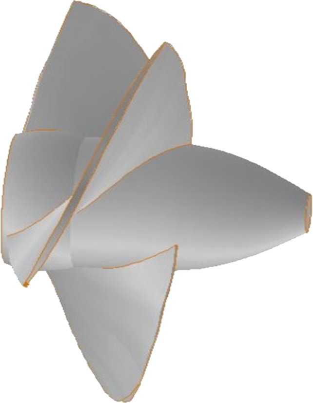
Runner model.

Near the Solid Wall Boundary. The velocity gradient of the viscous sublayer is high near the solid wall for turbulent flow. The high-Reynolds-number calculation model is no longer applicable. The gradient can be obtained using the wall function for flow near the wall.

Inlet Boundary. The inlet conduit imports the inlet boundary and uses the pressure-inlet boundary condition.

Outlet Boundary. The outlet conduit exports the outlet boundary and uses the pressure-outlet boundary condition.

3.3. Efficiency Calculation Method

Efficiency is an important parameter for measuring turbine energy performance.

Turbine output is the power output of the turbine shaft, commonly denoted by P and with kW for the units.

The turbine input power is the total energy flow through the turbine per unit time. The flow output is usually indicated by the symbol P_n:

P_{n} = γ Q H = 9.81 Q H (kW) .

(4)

A certain energy loss occurs as the water flows through the turbine. So the turbine output P is always smaller than the flow output P_n. The ratio of turbine output to water output is called the turbine efficiency and is indicated by η_t:

η_{t} = \frac{P}{P_{n}} .

(5)

4. Runner Optimization

Tubular-turbine blades have a 3D twisted leaf shape. In the work reported in this section, the flow component parameters were kept at the same values under the same calculation conditions to optimize the three aspects of the blade shape and to perform a CFD simulation using various models. The results obtained were analyzed for optimality.

4.1. Shape Optimization of Turbine Blade Edges

Figure 5 shows a schematic view of the modification; improved access to the turbine blade edge was achieved by changing the edge from straight to curved, as shown in Figure 4, which presents different single-blade diagrams for straight and curved edges.

Figure 4:

Turbine blade edge, schematic view.

Figure 5:

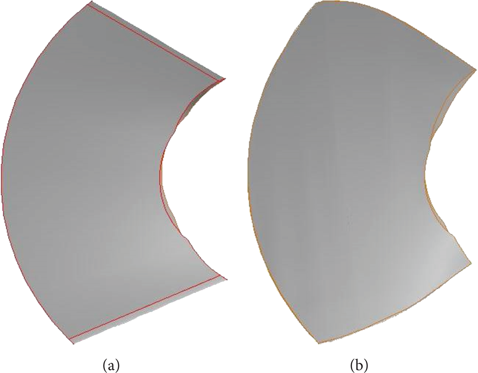
Single-blade diagram ((a) is a straight edge and (b) is a curved edge).

Numerical simulations of the two blade-edge shapes were performed under the positive operating mode (H = 2.5 m, guide-vane opening speed = 65%, and speed = 200 rpm), with results listed in Table 1. It is apparent that different blade edges have an impact on performance, although the overall efficiency slightly decreased. However, the turbine discharge increased significantly, with a substantial increase in output torque, which contributes greatly to improved output.

Table 1:

Calculated results for two kinds of blade-edge shapes.

Blade-edge shapes	Discharge (m³/s)	Torque (N M)	Efficiency (%)	Output (KW)

Straight edge	6.05	5909.23	83.36	123.74
Curved edge	9.38	9133.39	83.16	191.25

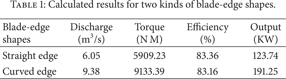
Table 2 shows the head loss of various components for the two blade-edge shapes. It is clear that the hydraulic losses in the runner segment with the curved edge were greatly reduced, but this segment led to the inlet conduit section, where the guide-vane segments and the outlet conduit segment increased the hydraulic losses. The additional losses entailed by these components diminished slightly the reduced hydraulic losses in the runner segments, which corresponded to the efficiency change of the two blade-edge shapes shown in Table 1. However, the discharge was greatly improved, which directly increased unit output.

Table 2:

Component hydraulic losses for different blade-edge shapes.

Blade-edge shape	Inlet conduit segment loss	Guide-vane segment loss	Runner segment loss	Outlet conduit segment loss

Straight	0.003	0.028	0.285	0.077
Curved	0.005	0.046	0.177	0.151

4.2. Blade Twist Angle Optimization

The blade twist angle directly affects flow capacity and torque and has a significant impact on efficiency and unit output. Different blade twist angles were therefore investigated. Before retrofit design, the blade twist angle was 5°; a decrease to 3° and increases to 7°, 9°, and 11° were examined, giving five twist-angle cases. Numerical simulation was performed with the five models under the same operating conditions (H = 2.5 m, guide-vane opening speed = 65%, and speed = 200 rpm), and the calculated results are shown in Tables 3 and 4.

Table 3:

Performance calculations for different blade twist angles under the positive power model.

Blade twist angle	Discharge (m³/s)	Torque (N M)	Efficiency (%)	Output (KW)

3°	5.85	5529.77	80.71	115.79
5°	6.05	5909.23	83.36	123.74
7°	9.38	9133.39	83.16	191.25
9°	9.15	8537.45	79.67	178.78
11°	8.54	7453.39	74.52	156.07

Table 4:

Performance calculations for different blade twist angles under the reverse power model.

Blade twist angle	Discharge (m³/s)	Torque (N M)	Efficiency (%)	Output (KW)

3°	5.58	4529.77	69.31	94.85
5°	6.46	5609.23	74.14	117.46
7°	8.39	8133.39	82.77	170.31
9°	7.55	7037.45	79.59	147.37
11°	6.78	6053.39	76.23	126.76

From Tables 3 and 4, when the blade twist angle = 7°, the efficiency and unit output have the largest values.

4.3. Optimization of the Distance between the Runner and the Guide Vanes

Figure 6 shows a three-dimensional model of the runner vanes and the runner. The distance between the two components, represented by the letter d, has a significant impact on efficiency and unit output. The runner diameter is denoted by r and has a fixed value. Simulated changes in d/r, which involve changing the distance between the guide vanes and the runner, were used to compare different blade locations, where d/r = 0.5, 0.75, 1.0, 1.25, 1.5, and 2, giving five different positions. Numerical simulations were performed with the five models under the same operating conditions (H = 2.5 m, guide-vane opening speed = 65%, and speed = 200 rpm), with the calculated results shown in Figures 7 and 8.

Figure 6:

Three-dimensional model of runner vanes and runner.

Figure 7:

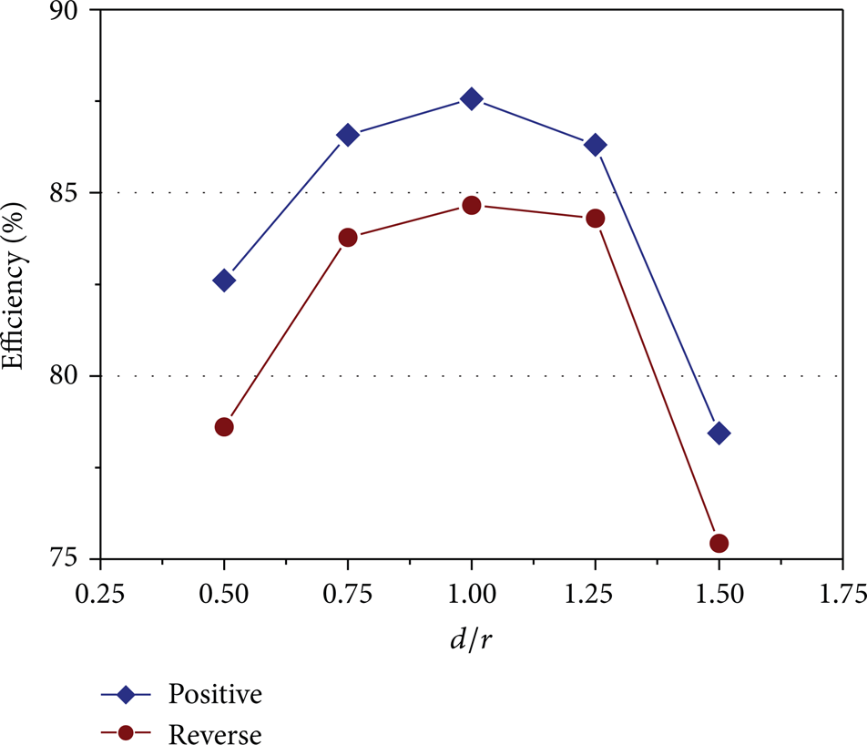
Efficiency versus d/r contribution plot for positive and reverse working conditions.

Figure 8:

Output versus d/r contribution plot for positive and reverse working conditions.

From Figures 7 and 8, it can be seen that when d/r = 0.75, 1.0, and 1.25, the runner efficiency and the output had higher values, indicating that the distance between the guide vane and the runner must not be too large or too small. In this situation, d/r = 0.75 was taken as the optimal value.

4.4. Analysis of Flow Pattern before and after Optimization

In the previous sections, three optimization aspects were considered, and optimal parameter values were integrated to achieve optimization improvements. Specifically, the curved blade-edge shape was chosen, the optimal blade twist angle was 7°, and d/r = 0.75. Numerical simulations should be performed to analyze flow patterns before and after optimization.

4.4.1. Static Pressure Distribution of the Blade

Figures 9 and 10, respectively, show the static pressure distributions before and after modification of the blade. The pressures gradually decreased in the flow direction on the whole, with the positive pressure greater than the back pressure, which had some influence on the positive pressure, but the difference was small. After the blade was improved, the low pressure was localized mainly in the middle of the turbine wheel hub.

Figure 9:

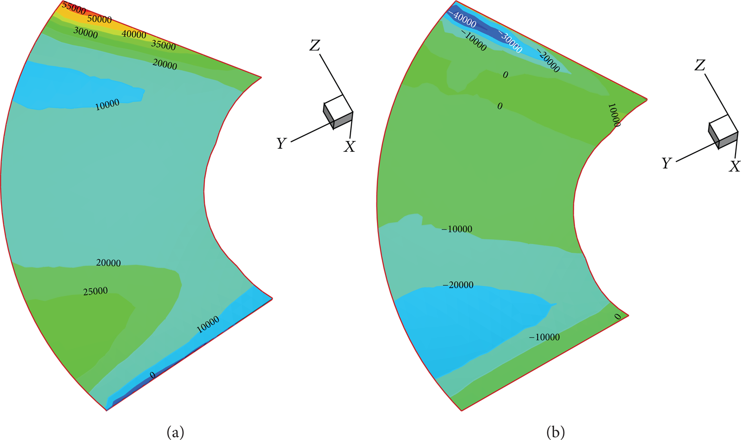
Static pressure distribution of blade before modification ((a) is the front face and (b) is the back face).

Figure 10:

Static pressure distribution of modified blade ((a) is the front face and (b) is the back face).

4.4.2. Surface Relative Velocity Distribution

Figures 11 and 12, respectively, show the front and back relative velocity distribution before and after modification. As is clear from the figure, both before and after blade retrofits, the water flow along the blade surface was smooth, with no turbulence, and the flow pattern was good.

Figure 11:

Relative velocity distribution (front (a) and back (b)) of blade before modification.

Figure 12:

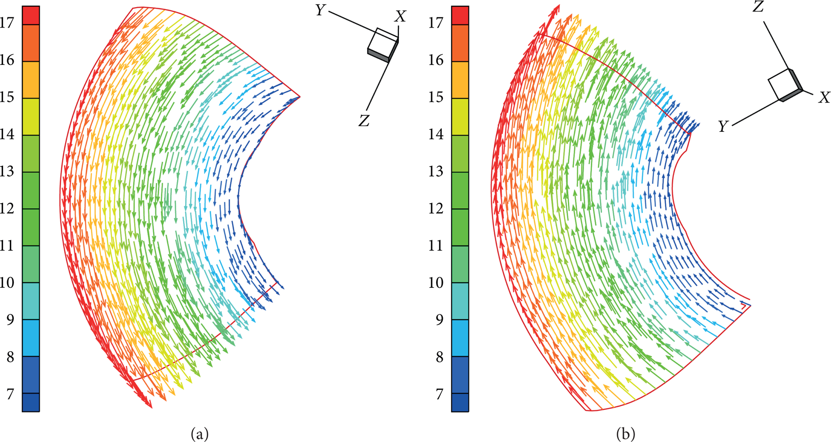
Relative velocity distribution (front (a) and back (b)) of modified blade.

5. Experiments

The hydraulic machinery multifunction test bench of Hohai University was used for the “211 Project” key construction projects. The test bench was designed and constructed according to standard DL446-91 “Turbine Model Acceptance Tests,” with an integrated test error less than or equal to 4%. The test bed is a vertical closed-loop system with a total capacity of 50 m³. The main equipment consists of the tail tank, pressure tank, electromagnetic water pump (or auxiliary pump), electric valve, manual butterfly valve, Φ500 pipes, and other components. The main parameters are as follows:

head: H = 0–20 m;

discharge: Q = 0–1 m³/s;

torque: M = 0–200 N • M;

speed: n = 0–2000 rpm.

Figure 13 provides a photograph of a guide vane. The masses of water around the guide vanes are an important part of the turbine system, and the flow energy loss in the water guide vanes will affect the efficiency of the turbine. By adjusting the guide vanes, unit load changes can be compensated for. A photograph of the runner model is shown in Figure 14. Using the wheeled test bench, forward and reverse efficiency and performance experiments could be carried out. The model test head was kept stable at H = 2.5 m; by adjusting the guide vane in steps from 30° to 85°, each guide vane could be kept stable for five minutes in each position to collect data. Statistics of the collected data and efficiency data calculated by numerical simulation under the same conditions are shown in Figures 15 –17.

Figure 13:

Photograph of guide vane.

Figure 14:

Photograph of turbine runner model.

Figure 15:

Discharge versus guide-vane opening curve.

Figure 16:

Efficiency versus discharge curve for the positive generation case.

Figure 17:

Efficiency versus discharge curve for the reverse generation case.

As shown in Figure 15, the discharge increases with guide-vane opening flow for both positive and reverse generation cases. When the guide vane reaches 70% open, the discharge does not increase any more under the positive condition because with further opening of the guide vane, the hydraulic losses increase so much that further increases in discharge cannot be achieved.

Figures 16 and 17 show that

numerical simulation results matched with experimental data very well;

the efficiency of the positive generation condition is slightly greater than that of the reverse condition;

the highest efficiency for positive generation was achieved at guide-vane opening = 60%, discharge = 8.5 m³/s, efficiency = 86.4%, and output = 186.5 kW. The highest efficiency for reverse generation was achieved at guide-vane opening = 75%, discharge = 7.87 m³/s, efficiency = 84.08%, and output = 163.5 kW.

6. Conclusion

The shaft tubular turbine is a form of tidal power station turbine which can provide bidirectional power with high efficiency. The turbine runner is the core component which converts water energy into mechanical energy. This paper has optimized the runner from three aspects using numerical simulation methods and verified the optimized runner design. From the hydraulic machinery multifunctional tests, the main conclusions are as follows.

Comparing the curved-edge and straight-edge blades under the same operating conditions, the efficiency changes a little, but the curved-edge blade can directly increase discharge capacity and output, meaning that the curved-edge blade is much better than the straight-edge blade.

Blade twist angle directly affects flow capacity and torque and has a significant impact on efficiency and unit output. According to the model used in this paper, when the blade twist angle = 7°, the bidirectional efficiency and unit output have the best values.

The optimized ratio d/r of the guide vanes and runner distances is (0.75–1.25) because when the ratio is too large or too small, the flow patterns between guide vane and runner are relatively poor.

When model tests of the optimized runner were carried out, by comparing the model test and numerical simulation results, it was found that the numerical simulation results matched the experimental data very well, which verified the correctness of the optimal results.

Footnotes

Acknowledgment

This work is supported by Special Funds for MRE: GHME2011CX02.

References

Yang

Zheng

, and Yan

, “Inlet passage's development and calculation of new tidal unit-shaft tubular turbine,” in Proceedings of the International Conference on Materials for Renewable Energy & Environment, 2012.

Chunxia

Yuan

, and Daqing

, “Development and optimization design of shaf tubular turbine with super low-head,” in Proceedings of the 26th IAHR Symposium on Hydraulic Machinery and Systems, 2012.

yuan

and Zaiming

, “Research on energy characteristics of bidirectional tubular turbine,” in Proceedings of the 5th Joint ASME/JSME Fluids Engineering (FEDSM '07), San Diego, Calif, USA, 2007.

Nai-Xing

and Yan-Ji

, “Numerical computation of 3-D turbulent flow in turbine cascade,” Chinese Science Bulletin, vol. 1, pp. 57–61, 2005.

yuan

and Zongyin

, “Technique on flow measurement and its application in low head and large discharge pump stations,” in Proceedings of the 5th Joint ASME/JSME Fluids Engineering, San Diego, Calif, USA, 2007.

Yang

Hao

Guo

, and Zhang

, “The research and design of vertical-shaft water turbine power generation device,” in Proceedings of the International Conference on Materials Science and Technology (ICMST 10), Trans Tech Publications, Jeju Island, Republic of Korea, December 2010.

Feng-Mei

Gang

, and Zhi-Min

, “Calculation method of fluid and structure interaction in a vertical-axis tidal current turbine,” Zhendong Yu Chongji/Journal of Vibration and Shock, vol. 32, no. 8, pp. 91–95, 104, 2013.

Obara

Morizane

, and Morel

, “Study on method of electricity and heat storage planning based on energy demand and tidal flow velocity forecasts for a tidal microgrid,” Applied Energy, vol. 111, pp. 358–373, 2013.

FuJun

, Computational Fluid Dynamics Analysis— CFD Software Principle and Application, Tsinghua University Press, Beijing, China, 2004.

10.

Xinfeng

yuan

Zhongxin

, and Minghui

, “Efficiency calculation and the vortex characteristics research of centrifugal pump,” in Proceedings of the 26th IAHR Symposium on Hydraulic Machinery, Beijing, China, August 2012.

11.

Fan

Zhou

, and Zhang

, “Optimization of household mini tubularturbines of shaft extension,” vol. 31, no. 5, pp. 260–265, 2012.

12.

Tan

Cao

, and Gui

, “Hydraulic design and pre-whirl regulation law of inlet guide vane for centrifugal pump,” Science China Technological Sciences, vol. 53, no. 8, pp. 2142–2151, 2010.

Optimization Study of Shaft Tubular Turbine in a Bidirectional Tidal Power Station

Abstract

1. Introduction

2. Working Principles

3. Numerical Simulation [8–12]

3.1. Basic Equations

3.2. Geometric Model and Boundary Conditions

3.3. Efficiency Calculation Method

4. Runner Optimization

4.1. Shape Optimization of Turbine Blade Edges

4.2. Blade Twist Angle Optimization

4.3. Optimization of the Distance between the Runner and the Guide Vanes

4.4. Analysis of Flow Pattern before and after Optimization

4.4.1. Static Pressure Distribution of the Blade

4.4.2. Surface Relative Velocity Distribution

5. Experiments

6. Conclusion

Footnotes

Acknowledgment

References

3. Numerical Simulation [8 –12]