Sage Journals: Discover world-class research

Abstract

This study presents the flexible-body dynamic analysis and simulated stress recovery of vehicle components to predict their lifetime when maneuvering on an uneven random road. The subject of this study was an all-terrain vehicle (ATV). The body frame and suspension system were modeled as flexible elements for multibody dynamic simulation. The simulations in this study revealed the stress from the flexible elements and predicted the component fatigue life using the retrieved stresses. This approach considers the interaction between dynamic forces and structure deformation and achieves more accurate structure stress prediction and fatigue life prediction.

1. Introduction

Fatigue is one of the major concerns in automotive engineering. The structure and components of a vehicle are constantly under cyclic loading, and especially on rough roads. This could cause the fatigue failure of the structure or components. Ohchida [1] showed that 60% of machine equipment failures are caused by component fatigue. Therefore, a reliable method for predicting the potential fatigue failures of vehicle components is highly desirable. In the design cycle of automotive vehicles, the majority of automotive manufacturers use empirical methods or dynamic simulations to predict the component and structure loadings [2]. The FEA model was designed to predict the stress of components and fatigue failure [3]. However, the FEA analysis process does not consider the effects of the dynamic loads caused by structural deformations. The dynamic loading that occurs when the vehicle is running can cause structural deformation, which in turn may affect load conditions and further change the stress of components. Thus, dynamic analysis with a rigid body system is insufficient. The dynamic loading changes caused by structural deformation should be considered in structure and component stress analysis. Cuadrado et al. [4] presented flexible-body dynamic simulations considering the effects of structural deformation and can therefore predict more accurate loads and stresses of the vehicle components than the general rigid-body simulation can. The good correlation between simulation and experimental results was presented as well in their study. Some studies have focused on vehicle components by modeling them as flexible elements in multi-body dynamic simulation. Moon et al. [5] presented a taper leaf spring with hysteretic characteristics. This study developed a flexible multi-body dynamic simulation to interface the leaf spring finite-element model and computation model and correlated simulation and experimental results. Shabana and Sany [6] presented a rolling contact theory with multi-body dynamics to simulate the effects because of the structural flexibility of the vehicle component and track. Zhu et al. [7] predicted the fatigue life of a truck frame. They modeled the frame as a flexible element and the vehicle system as rigid multi-body dynamic model. Yang et al. [8] predicted the fatigue life of a wheel by simulating the EMU wheel as a flexible body in multi-body simulations. Rathod et al. [9] presented a multi-body railroad vehicle system that accounted for the dynamic coupling between a 3D wheel and the rail structure flexibility. However, these studies did not include the deformation of the entire vehicle structure.

This study uses ADAMS to perform flexible-body dynamic simulation and models all structural components as flexible elements. The stress history of the structure was then retrieved from the dynamic simulation for fatigue calculation.

The remaining sections are as follows: the theoretical background of the flexible-body dynamics and fatigue analysis, the simulation model, the simulation results, and the conclusion.

2. Theory Background

2.1. Equations of Flexible-Body Dynamics

In equations of motion, the linear deformation of a structure can be represented by the combination of mode shapes and mode coordinates as follows:

u = \sum_{i = 1}^{M} φ_{i} q_{i},

(1)

where φ is the mode shape and q is the mode coordinate.

With the Cartesian coordinate (x, y, z), Euler's angle (ψ, θ, φ), mode coordinate q, and the generalized coordinates of the flexible element can be expressed as follows:

ξ = (\begin{pmatrix} x \\ ψ \\ q \end{pmatrix}) = {\begin{Bmatrix} x \\ y \\ z \\ ψ \\ θ \\ φ \\ q_{i} \end{Bmatrix}}, (i = 1,2, 3, \dots, M) .

(2)

The position on the deformed body is written as

r_{i} = x + A (S_{i} + φ_{i} q),

(3)

where A is the transformation matrix between global coordinates and the body local coordinates. The term S_i represents the position in the body before deformation, and φ_i is the mode shape matrix.

From the position, the velocity of the deformed body is

v_{i} = \frac{d r_{i}}{d t} = \frac{d x}{d t} + \frac{d A}{d t} (s_{i} + φ_{i} q) + A \frac{d (s_{i} + φ_{i} q)}{d t} = \dot{x} - A ({\tilde{s}}_{i} + {\tilde{φ}}_{i} q) ω + A φ_{i} \dot{q} = | F - A ({\tilde{s}}_{i} + {\tilde{φ}}_{i} q) B + A φ_{i} | \dot{ξ} .

(4)

The term ω is the angular velocity vector of the body coordinate, and F is the transfer matrix between the time derivative of Euler's angle and the angular velocity.

The kinematic energy of the body is

T = \frac{1}{2} \int ρ v^{T} v d V \approx \frac{1}{2} \sum_{i = 1}^{N} (m_{i} v_{i}^{T} v_{i} + ω_{i}^{T} I_{i} ω_{i}) = \frac{1}{2} {\dot{ξ}}^{T} M (ξ) \dot{ξ},

(5)

where m_i and I_i represent the modal mass and modal inertia of moving body, respectively.

The mass matrix of flexible body, M, can be expressed as

M (ξ) = [\begin{bmatrix} M_{t t} & M_{t r} & M_{t m} \\ M_{t r}^{T} & M_{r r} & M_{r m} \\ M_{t m} & M_{r m}^{T} & M_{m m} \end{bmatrix}],

(6)

where t, r, and m represent the translational, rotational, and modal degrees of freedom, respectively.

The stiffness matrix of the flexible body, K, is relatively simple because there is no rigid body contribution:

K (ξ) = [\begin{bmatrix} K_{t t} & K_{t r} & K_{t m} \\ K_{t r}^{T} & K_{r r} & K_{r m} \\ K_{t m}^{T} & K_{r m}^{T} & K_{m m} \end{bmatrix}] = [\begin{bmatrix} 0 & 0 & 0 \\ 0 & 0 & 0 \\ 0 & 0 & K_{m m} \end{bmatrix}] .

(7)

The equations of motion with a Lagrange multiplier can be written as follows:

M \ddot{ξ} + \dot{M} \dot{ξ} - \frac{1}{2} {[\frac{\partial M}{\partial ξ} \dot{ξ}]}^{T} \dot{ξ} + K ξ + f_{g} + D \dot{ξ} + {[\frac{\partial ψ}{\partial ξ}]}^{T} λ = Q .

(8)

The term D is the modal damping matrix, and Kξ and $D \dot{ξ}$ , respectively, represent the structural internal force caused by the elastic deformation and velocity. The term λ is the Lagrange multiplier, f_g is the structure weight, and Q is the external force.

The strain and stress can be retrieved using the mode coordinate [10]. This study calculates the stress in the structure using the modal stress recovery technique:

\begin{matrix} {ε} = [H] {x}, \\ {σ} = [E] {ε} . \end{matrix}

(9)

The term {σ} is the stress vector, {ε} is the strain vector, and [H] is the finite-element geometric deformation-to-strain matrix. The term [E] is the material property matrix.

2.2. Fatigue Prediction

Metal material under cycling stress can fail even when the stress is under the ultimate stress limit. The relationship between fatigue stress and life cycle is usually represented by a stress-cycles curve (S-N diagram). For steel, a cycle life greater than 10⁶ is treated as a lasting life, and the stress corresponding to a 10⁶ cycle is the endurance limit S_e [11].

The S-N diagram is plotted in log scale, and the formula of S-N curve can be simplified as

\log S_{f} = \log a + b \log N ⟹ S_{f} = a N^{b},

(10)

where b is the slop of curve and N is the life cycle.

During vehicle maneuvering, the structural stress is fluctuating. The amplitude of stress variation varies with the driving and road conditions. The rain-flow counting technique can be applied to measure different stress variations during driving. The Palmgrem-Miner cycle-ratio summation rule can then be used to accumulate the damages of various loads and cycles:

\sum_{i = 1}^{i = N} \frac{n_{i}}{N_{f i}} = Damage,

(11)

where n_i is the number of cycles at the change of stress amplitude (Δσ_i) and N_ft is the number of cycles until failure at the change of stress amplitude (Δσ_i). The “Damage” parameter usually ranges from 0.7 to 2.2. When the accumulated damage is larger than the “Damage” parameter, the component fails [12].

3. Vehicle Model

The object of research in this study is a dune buggy. Figure 1 shows the geometric model based on the measurement on the vehicle structure. For each component of vehicle structure, MSC Nastran was used to perform modal analysis, and MSC Patran was used to process finite-element models and modal analysis data to create flexible elements for dynamic simulation [13]. These elements were imported to the vehicle model to assemble the whole vehicle. Then, we used ADAMS to perform the flexible-body dynamic simulations [14] and determine the stress generated by random road maneuvers.

Figure 1:

Vehicle structure and suspension frames.

3.1. Components

The structure of vehicle model included three primary parts: the body frame, the front suspension, and the rear suspension (Figure 2). The powertrain and passenger weights were attached to the structure, and the total weight of vehicle was 423 kg. All the structure components were modeled as a flexible body. The tires were simulated as force elements in dynamic simulation [14]. Figure 2 shows the connecting joint and forces applied between components [14, 15], and Table 1 shows material properties of the frame [16].

Table 1:

Material property of vehicle structure.

Property	Steel 1015	Steel 1018

Elastic modulus (MPa)	2.07E05	2.07E05
Poisson ratio	0.29	0.29
Density (ton/mm³)	7.9E – 09	7.9E – 09
Ultimate strength (MPa)	414	455

Figure 2:

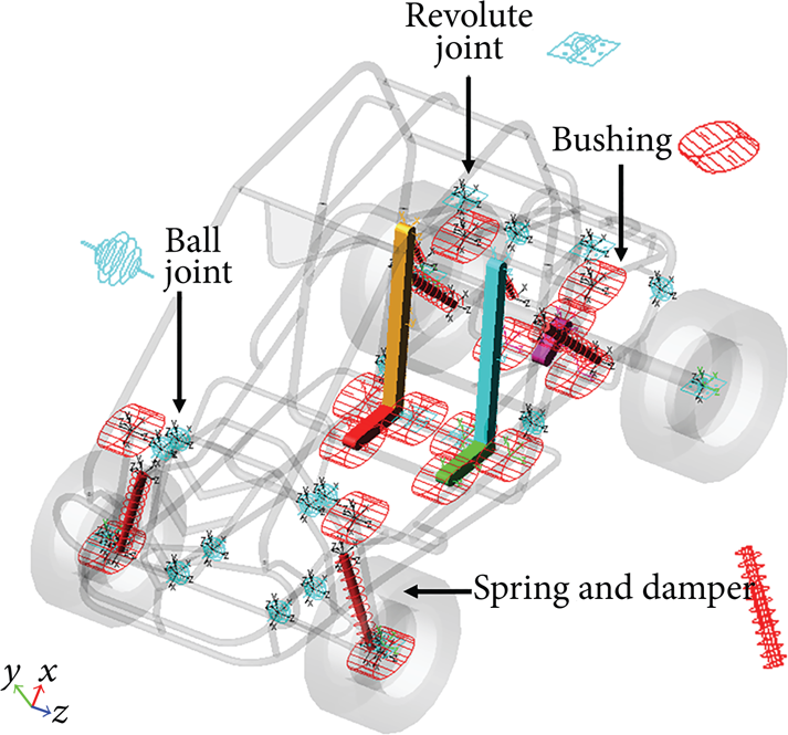
Assembled vehicle and connecting joints and forces.

In addition to the weight of the vehicle structure and the driveline, two dummies weighing 80 kg each were modeled and seated on the vehicle structure. The dummies were modeled as two parts (the upper torso; pelvis and legs) [10], which were connected with a revolute joint. The upper torso, including the seat back, and the pelvis, including the seat, were attached to the vehicle structure by springs and dampers. Table 2 lists the spring stiffness and damping coefficient. The driveline was seated on the engine mounts, and the engine mounts were modeled as rubber bushings. Table 2 lists the parameters.

Table 2:

Properties of dummies and driveline.

	Mass (kg)	Spring stiffness (N/mm)	Damping coefficient (N-s/mm)

Upper torso (including seat back)	45	10	0.4
Hips and leg (including seat)	35	15	0.2
Powertrain	40	52	0.12

3.2. Tire and Road Models

The simulations in this study modeled tires as force elements, and these tire models included the tire mass and inertia. The simulations in this study use the Fiala tire model, which was designed for vertical and longitudinal motion. Table 3 presents the tire parameters.

Table 3:

Tire parameters.

Property	Front tire	Rear tire

Tire model	Fiala tire type	Fiala tire type
Mass (kg)	10	11
Moment of inertia (kg-mm²)	Ixx, Iyy: 8E5; Izz: 16E5	Ixx, Iyy: 8E5; Izz: 16E5
Tire radius (mm)	254	280
Tread width (mm)	200	200

For simulation road condition, this study applies a random 2D surface (Figure 3).

Figure 3:

2D random road profile.

4. Simulation and Result

In the simulation, the vehicle maneuvered in straight runs over a random uneven surface. The vehicle accelerated from standing still, and the data for analysis was collected when it reached a constant speed of 50 km/h. The duration of data collecting was 10 s. Several thicknesses of the structure frame tube were applied in the simulation: 1 mm, 1.5 mm, 2 mm, and 2.5 mm.

4.1. Dynamic Simulation

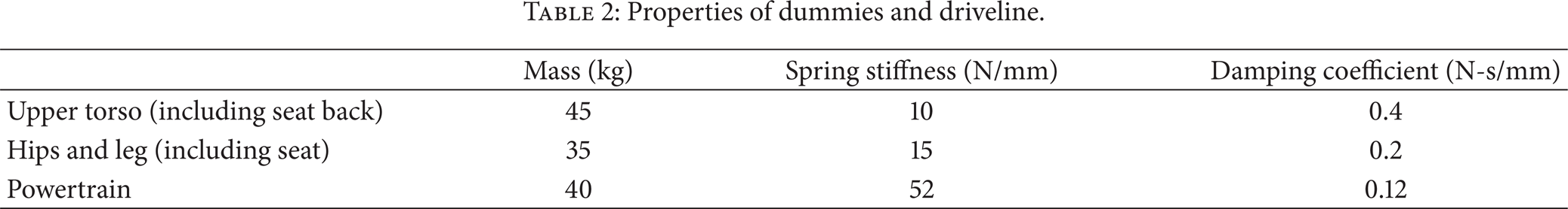
In flexible-body dynamic simulation, ADAMS can retrieve the structural stress which could be applied to failure or fatigue analysis. Figure 4 shows the highest stress locations during the dynamic simulation. Table 4 shows the maximum von Misses stress of these locations in uneven random road simulations.

Table 4:

Structure stress retrieved from flexible body dynamic simulation.

Frame tube thickness (mm)	Road surface	Max. stress grid point	Max. stress (MPa)

1	Flat	582887	215.36
1	Random	585076	498.30

1.5	Flat	582887	163.08
1.5	Random	586151	430.28

2	Flat	582887	137.87
2	Random	586151	361.84

2.5	Flat	582887	105.33
2.5	Random	585079	347.21

Figure 4:

Highest stress locations at random road simulation.

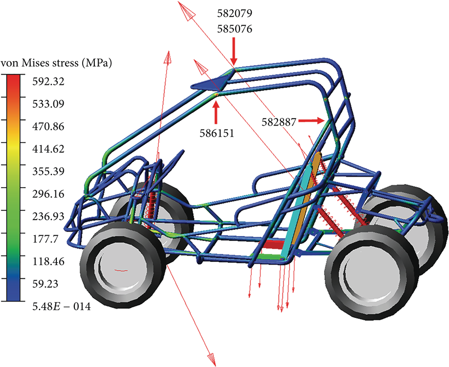
To compare the differences in dynamic load running on an uneven road surface, this study created both rigid-body and flexible-body models. Because the rigid-body dynamic simulation cannot determine the structural stress, the maximum rear suspension joint forces were used to present the difference between these two types of simulation (Table 5). Figure 5 shows the joint locations. The frame tube thickness of the model was 2.0 mm in this simulation.

Table 5:

Joint force comparison between flexible-body and rigid-body simulation.

Frame tube thickness (mm)	Right and left jointsaverage force at rear suspension (N)	Difference

Flexible-body model	623.01	—
Rigid-body model	758.09	21.7%

Figure 5:

Joint locations.

In addition to the suspension and tire elements, the flexible element in the vehicle structure also absorbed part of dynamic energy during the uneven road simulation. Thus, the joint force of the flexible-body model was smaller than that of the rigid-body model during the simulation.

4.2. Fatigue Analysis

The FEM model in this study adopts several thicknesses of the frame tube. The flexible elements were built based on these models, and flexible-body dynamic simulations were run with different tube thicknesses. The tube thicknesses were 1 mm, 1.5 mm, 2 mm, and 2.5 mm. The maximum stress was retrieved and plotted in a stress-time curve. Figure 6 shows the stress history of the structure with a 2.5 mm tube thickness in 10 s simulation at a constant speed of 50 km/h.

Figure 6:

Stress history of the max. stress grid point (585079).

The rainflow counting method was applied to the stress history curve, and the stress cycle number of different stress amplitudes was used for fatigue analysis. Figure 7 shows the stress range and cumulative cycle number of different frame tube thicknesses.

Figure 7:

Cumulative cycle number of different frame tube thicknesses.

Based on the stress cycle and material S-N diagram, the structural life can be predicted using the Miner rule. Using a 10 s simulation cycle, Table 6 presents the structural life of different frame tube thicknesses. This duration time and the maximum stress position listed in Table 4 show that the structure connecting points of two or more structure members are the most vulnerable to fatigue damage.

Table 6:

Fatigue analysis of different tube thicknesses.

Tube thickness	1 mm	1.5 mm	2 mm	2.5 mm

Cycle number	Less than 1	N_f = 218	N_f = 1265	N_f = 2780

5. Conclusions

Conventional analysis methods model the vehicle body as a rigid body in dynamic simulations. In this case, the dynamic energy passing from the tire running over an uneven road can only be absorbed and damped by tires, springs, and dampers in suspension, and bushings. After this rigid body dynamic simulation, the component load was applied to a finite-element model to determine the structural stress of the component for further analysis. The approach used in this paper is different from the conventional one. The dynamic model in this study uses flexible bodies. The advantage of using flexible-body dynamic simulation is that it simulates structural stresses in dynamic analysis and can be retrieved through the simulation. The dynamic response considers the effect of structural deformation. This provides more realistic and better prediction, especially for not-so-rigid vehicle structures. The structure can also absorb part of the energy. Thus, the loads at joints were smaller compared with the loads obtained in rigid-body simulation.

The stress received from flexible dynamic analysis can be used in fatigue analysis. The structure connecting points where two or more structure members were welded together appeared to be the most vulnerable to fatigue damage. Therefore, these points should be reinforced during structure design and assembly to increase the expected lifetime.

Vehicle fatigue testing is costly and time consuming. Flexible-body dynamic simulations can assist in the life prediction of vehicle structures and components. The proposed analysis tool can shorten the design cycle and can reduce vehicle development cost and time.

Footnotes

Notations

References

Ohchida

, “Analysis of service failures of Hitachi products 1970–1975,” Hitachi Company Report, 1979.

, and Dong

, “Dynamic modeling and virtual test of a new all terrain off-road vehicle,” Applied Mechanics and Materials, vol. 86, pp. 125–128, 2011.

Miao

B. R.

Zhang

W. H.

Zhang

L. M.

Zhu

, and Yin

H. T.

, “Research of modern railway vehicle structure fatigue design method based on multibody dynamic simulation,” Advanced Materials Research, vol. 118–120, pp. 327–331, 2010.

Cuadrado

Gutierrez

Naya

M. A.

, and Gonzalez

, “Experimental validation of a flexible MBS dynamic formulation through comparison between measured and calculated stresses on a prototype car,” Multibody System Dynamics, vol. 11, no. 2, pp. 147–166, 2004.

Moon

I.-D.

Yoon

H.-S.

, and Oh

C.-Y.

, “A flexible multibody dynamic model for analyzing the hysteretic characteristics and the dynamic stress of a taper leaf spring,” Journal of Mechanical Science and Technology, vol. 20, no. 10, pp. 1638–1645, 2006.

Shabana

A. A.

and Sany

J. R.

, “A survey of rail vehicle track simulations and flexible multibody dynamics,” Nonlinear Dynamics, vol. 26, no. 2, pp. 179–210, 2001.

Zhu

Xiao

, and Li

, “Vehicle frame fatigue life prediction based on finite element and multibody dynamic,” Applied Mechanics and Materials, vol. 141, no. 1, pp. 578–585, 2012.

Yang

Shi

Zhang

, and Zhang

, “The fatigue life simulation of the wheel of CHR3 EMU in random loading,” Advanced Materials Research, vol. 430–432, pp. 1424–1427, 2012.

Rathod

Chamorro

Escalona

J. L.

El-Sibaie

, and Shabana

A. A.

, “Validation of three-dimensional multibody system approach for modelling track flexibility,” Proceedings of the Institution of Mechanical Engineers K, vol. 223, no. 4, pp. 269–282, 2010.

10.

Wasfy

T. M.

and Noor

A. K.

, “Computational strategies for flexible multibody systems,” Applied Mechanics Reviews, vol. 56, no. 6, pp. 553–613, 2003.

11.

Yao

, Structure Fatigue Analysis, Defence Inductry Publisher, 2003.

12.

Shigley

J. E.

and Mischke

C. R.

, Mechanical Engineering Design, McGraw Hill, 2010.

13.

MSC Software, Nastran User's Manual, MSC Software, Newport Beach, Calif, USA, 2010.

14.

MSC Software, MDAdams. ADAMS User's Manual, MSC Software, Newport Beach, Calif, USA, 2010.

15.

Azadi

Behzadipour

, and Faulkner

, “Performance analysis of a semi-active mount made by a new variable stiffness spring,” Journal of Sound and Vibration, vol. 330, no. 12, pp. 2733–2746, 2011.

16.

Hibbeler

R. C.

, Mechanics of Materials, Prentice Hall, 2010.

All Terrain Vehicle Flexible Multibody Dynamic Simulation for Fatigue Prediction

Abstract

1. Introduction

2. Theory Background

2.1. Equations of Flexible-Body Dynamics

2.2. Fatigue Prediction

3. Vehicle Model

3.1. Components

3.2. Tire and Road Models

4. Simulation and Result

4.1. Dynamic Simulation

4.2. Fatigue Analysis

5. Conclusions

Footnotes

Notations

References