A Nonlocal Finite Element Approach to Nanobeams

Abstract

This paper presents a consistent derivation of a new nonlocal finite element procedure in the framework of continuum mechanics and nonlocal thermodynamics for the analysis of bending of nanobeams under transverse loads. This approach is able to provide the overall performance and the influence of specific parameters in the behavior of nanobeams and it is also able to deal with nanomechanical systems by solving a reduced number of algebraic equations. An example shows that the proposed nonlocal finite element procedure, using a mesh composed by only four elements of equal size, provides the exact values in terms of transversal displacement and bending of the nanobeam.

1. Introduction

Carbon nanotubes (CNTs) play a very significant role in many fields of nanotechnology, nanoscience, and nanoengineering and have high applications in nanocomposites, nanoelectronics, and nano-electromechanical systems and devices. Therefore, a thorough understanding of their nanomechanical properties is necessary for designing nanosystems and nanodevices [1].

Two main approaches for the analysis of CNTs can be followed: atomic modeling and continuum modelling. The former approach includes molecular dynamics simulations which consider each individual molecule and its mechanical or chemical mutual interactions [2]. As a consequence, the computational effort is extremely time consuming and the method is restricted to systems with a limited number of molecules or atoms. The latter approach is considered in this paper since it is more efficient from the analytical and computational point of view, see, for example, [3, 4].

Nonlocal effects have been introduced in the framework of nonlocal continuum theories by Eringen [5, 6]. Then gradient and integral approaches have been extensively applied to analyse localization phenomena, size-dependent effects, plasticity, and damage problems [7–11]. However several continuum models have been developed to analyse CNTs in terms of classical (local) models, see, for example, [12].

Since size-dependent effects are fundamental in CNTs, a nonlocal version of the classical Euler-Bernoulli beam is adopted in this paper and the effects of the nonlocalities on displacements and bending are investigated by using a consistent nonlocal thermodynamic approach.

A new nonlocal finite element model for nanobeams is then developed starting from a suitable variational statement obtained from the nonlocal thermodynamic analysis. The proposed procedure can be easily extended to different models of elastic nanobeams or to two-dimensional nanomodels.

Moreover, the use of the classical beam finite element for the analysis of the transversal deflection of the Euler-Bernoulli beam [13] is not adequate for the proposed nonlocal finite element problem. Accordingly the nodal finite element parameters of the beam are enhanced by introducing an additional parameter associated with the second derivative of the transversal displacement. The resulting element is termed enhanced finite element (EFE).

Exact equilibrium conditions and higher-order differential governing equation with the corresponding higher-order nonlocal boundary conditions are derived according to the thermodynamic requirements following the framework proposed in [14]. The exact solution has been used as a benchmark for the enhanced finite element analysis.

A nanobeam under a uniformly distributed transverse load is considered. The numerical solution is obtained by the recourse to the proposed nonlocal EFE procedure and the method shows no pathological behaviors such as mesh dependence, numerical instability, or boundary effects. A mesh composed of only n = 4 elements of equal size provides the exact solution in terms of displacement and bending moment.

The EFE procedure shows that the presence of a nonlocal effect tends to induce higher stiffness for nanobeams and the stiffness is enhanced with increasing nonlocal nanoscale effect.

2. A Nonlocal Elastic Model

Assuming that there is no heat input due to radiation or conduction, the absolute temperature and the density of mass are constant; the first law of thermodynamics, see, for example, [15], for isothermal processes and for a nonlocal behaviour can be formulated as follows:

${\int }_{\Omega }\rightharpoonup \stackrel{.}{e}\hspace{0.17em}d\mathbf{x}={\int }_{\Omega }\rightharpoonup \stackrel{-}{\mathit{\sigma }}*\stackrel{.}{\mathbf{∊}}d\mathbf{x}.$

(1)

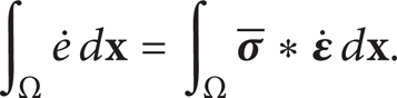
The internal energy density e depends on the strain tensor ε and entropy s, and a superimposed dot means time derivative. The energy balance in (1) can be written pointwise in the body domain Ω in the form [16]

$\stackrel{.}{e}=\stackrel{-}{\mathit{\sigma }}*\stackrel{.}{\mathbf{∊}}+P,$

(2)

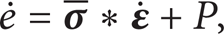
where P is the nonlocality residual function which takes into account the energy exchanges between neighbor particles [17]. The residual P fulfils the insulation condition

${\int }_{\Omega }\rightharpoonup Pd\mathbf{x}=\mathrm{0},$

(3)

since the body is a thermodynamically isolated system with reference to energy exchanges due to nonlocality.

The second principle of thermodynamics for isothermal processes in the nonlocal context is written in its local form [18] as follows:

$D=\stackrel{.}{s}T\ge \mathrm{0},$

(4)

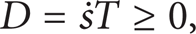
everywhere in Ω where $\mathrm{\hspace{0.17em}\hspace{0.17em}}\stackrel{.}{s}\mathrm{\hspace{0.17em}\hspace{0.17em}}$ is the internal entropy production rate per unit volume and D is the dissipation. The Helmholtz free energy φ (ε, T) is defined by means of the Legendre transform φ = e – sT so that, using the relation (2), the dissipation at a given point of the body is given in the following form:

$D=\stackrel{-}{\mathit{\sigma }}*\stackrel{.}{\mathbf{∊}}-\stackrel{.}{\phi }+P\ge \mathrm{0}.$

(5)

Note that (5) represents the nonlocal counterpart of the Clausius-Duhem inequality for isothermal processes and the nonnegativeness of the dissipation is guaranteed by the presence of the nonlocality residual function.

The body energy dissipation ℰ is given by integrating the relation (5) to get

$ℰ={\int }_{\Omega }\rightharpoonup \stackrel{-}{\mathit{\sigma }}*\stackrel{.}{\mathbf{∊}}d\mathbf{x}-{\int }_{\Omega }\rightharpoonup \stackrel{.}{\phi }d\mathbf{x}={\int }_{\Omega }^{}\stackrel{-}{\mathit{\sigma }}*\stackrel{.}{\mathbf{∊}}d\mathbf{x}-{\int }_{\Omega }^{}{d}_{\mathbf{∊}}\phi \left(\mathbf{∊}\right)*\stackrel{.}{\mathbf{∊}}d\mathbf{x}\ge \mathrm{0},$

(6)

which must hold for any admissible deformation mechanism so that, following widely used arguments, the nonlocal elastic state law is obtained as follows:

$\stackrel{-}{\mathit{\sigma }}=d_{\mathbf{∊}}\phi \left(\mathbf{∊}\right).$

(7)

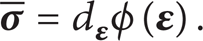
Accordingly the body energy dissipation ℰ vanishes and also the dissipation is pointwise vanishing; that is, D = 0, since (5) can be viewed as the nonnegative integrand of (6).

2.1. A Nonlocal Elastic Model of Nanobeams

Let us consider a thin nanobeam with length L, cross sectional area A, and Young's modulus E which is subjected to an external distributed transverse load p(z) as shown in Figure 1.

Figure 1:

Geometry and coordinate system of the beam.

The Euler-Bernoulli beam theory is adopted where a straight line normal to the midplane before deformation remains straight and perpendicular to the deflected midplane after deformation.

The axial elongation ε due to transverse displacements v of the nanobeam is given by $\mathrm{\hspace{0.17em}\hspace{0.17em}}\epsilon =-v^{(\mathrm{2})}y\mathrm{\hspace{0.17em}\hspace{0.17em}}$ where $\mathrm{\hspace{0.17em}\hspace{0.17em}}{v}^{(\mathrm{2})}\mathrm{\hspace{0.17em}\hspace{0.17em}}$ is the second derivative along the nanobeam axis of the transversal displacement field v and y is the bending axis. The superposed apex (·)⁽ⁿ⁾ denotes the n-th derivative of (·) with respect to the nanobeam axis z.

Nonlocality due to long range interactions arising in an elastic structure can be provided in terms of an integral relation which yields an integral constitutive relation [19]. An alternative approach, see [6, 20], is followed in this paper where the nonlocality is expressed in terms of a differential relation so that the corresponding constitutive relation turns out to be in a differential form.

The elastic energy for the nanobeams is defined according to the following expression:

$\hspace{0.17em}\phi \left(∊,{∊}^{\left(\mathrm{1}\right)}\right)=\frac{\mathrm{1}}{\mathrm{2}}E{∊}^{\mathrm{2}}+{\left(e_{0}a\right)}^{\mathrm{2}}E{∊}^{{\left(\mathrm{1}\right)}^{\mathrm{2}}},$

(8)

where a is an internal characteristic length (e.g., lattice parameter, C–C bond length, or granular distance) and e₀ is a material constant. The magnitude of e₀ can be determined experimentally or approximated by matching the dispersion curves of plane waves with those of atomic lattice dynamics. Classical elasticity for continuum mechanics is recovered in the limit of vanishing nonlocal nanoscale; that is (e₀a) → 0.

In the sequel, the variational relation among the bending moments and the displacement field, following from the elastic energy (8), is explicitly recovered since it is the starting point for the nonlocal FE analysis.

The vanishing of the body energy dissipation (6) together with the expression (8) provides the relation

${\int }_{\Omega }^{}\stackrel{-}{\sigma }*\stackrel{.}{∊}dz-{\int }_{\Omega }^{}{d}_{∊}\phi *\stackrel{.}{∊}dz-{\int }_{\Omega }^{}{d}_{{∊}^{\left(\mathrm{1}\right)}}\phi *{\stackrel{.}{∊}}^{\left(\mathrm{1}\right)}dz={\int }_{\Omega }^{}\stackrel{-}{\sigma }*\stackrel{.}{∊}dz-{\int }_{\Omega }^{}{\sigma }_0*\stackrel{.}{∊}dz-{\int }_{\Omega }^{}{\sigma }_{\mathrm{1}}*{\stackrel{.}{∊}}^{\left(\mathrm{1}\right)}dz=\mathrm{0},$

(9)

where $\mathrm{\hspace{0.17em}\hspace{0.17em}}\Omega =[\mathrm{0},L]\mathrm{\hspace{0.17em}\hspace{0.17em}}$ so that the following constitutive relations hold:

$\begin{array}{c}{\sigma }_0=d_{∊}\phi \left(∊,{∊}^{\left(\mathrm{1}\right)}\right)=E∊,\\ {\sigma }_{\mathrm{1}}=d_{{∊}^{\left(\mathrm{1}\right)}}\phi \left(∊,{∊}^{\left(\mathrm{1}\right)}\right)=E{\left(e_{0}a\right)}^{\mathrm{2}}{∊}^{\left(\mathrm{1}\right)}.\end{array}$

(10)

By inserting the expression of the beam axial elongation $\mathrm{\hspace{0.17em}\hspace{0.17em}}\stackrel{.}{\epsilon }\mathrm{\hspace{0.17em}\hspace{0.17em}}$ and of its derivative $\mathrm{\hspace{0.17em}\hspace{0.17em}}{\stackrel{.}{\epsilon }}^{(\mathrm{1})}\mathrm{\hspace{0.17em}\hspace{0.17em}}$ in the energy dissipation (9), after some rearrangements of the various terms and denoting by M, M₀, and M₁ the bending moment associated with the stresses $\mathrm{\hspace{0.17em}\hspace{0.17em}}\stackrel{-}{\sigma }$ , σ₀, and σ₁ as follows:

$M={\int }_{\Omega }^{}\stackrel{-}{\sigma }ydz,M_i={\int }_{\Omega }^{}{\sigma }_{i}ydz,\hspace{1em}i=\left\{\mathrm{0,1}\right\},$

(11)

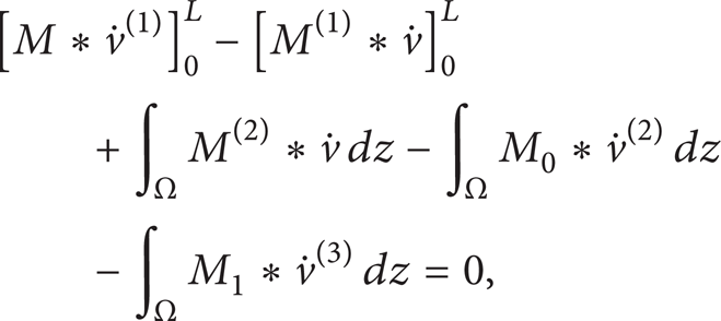
a more explicit expression (see Appendix A) can be given to the energy dissipation (9) in the following form:

${\int }_{\Omega }^{}M*{\stackrel{.}{v}}^{\left(\mathrm{2}\right)}dz-{\int }_{\Omega }^{}{M}_0*{\stackrel{.}{v}}^{\left(\mathrm{2}\right)}dz-{\int }_{\Omega }^{}{M}_{\mathrm{1}}*{\stackrel{.}{v}}^{\left(\mathrm{3}\right)}dz=\mathrm{0}.$

(12)

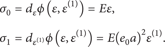
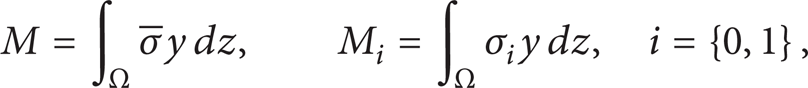
It is worth noting that the bending moments M _i , with i = {0,1}, can be expressed in terms of the transversal displacement field v as follows:

$\begin{array}{c}{M}_0={\int }_{\Omega }^{}E∊ydz=-E{\stackrel{.}{v}}^{\left(\mathrm{2}\right)}{\int }_{\Omega }^{}{y}^{\mathrm{2}}dz=-EJ{\stackrel{.}{v}}^{\left(\mathrm{2}\right)},\\ M_{\mathrm{1}}={\int }_{\Omega }^{}E{\left(e_{0}a\right)}^{\mathrm{2}}{∊}^{\left(\mathrm{1}\right)}ydz=-E{\left(e_{0}a\right)}^{\mathrm{2}}{\stackrel{.}{v}}^{\left(\mathrm{3}\right)}{\int }_{\Omega }^{}{y}^{\mathrm{2}}dz=-EJ{\left(e_{0}a\right)}^{\mathrm{2}}{\stackrel{.}{v}}^{\left(\mathrm{3}\right)},\end{array}$

(13)

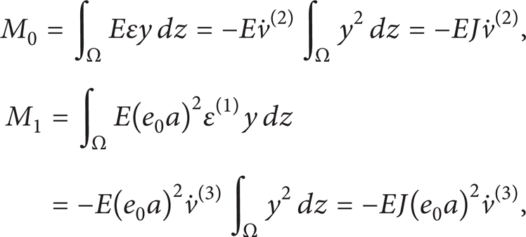
where EJ is the beam bending stiffness. Further, equilibrium considerations produce the usual results as follows:

$\begin{array}{c}{T}^{\left(\mathrm{1}\right)}\left(z\right)=-p\left(z\right),M^{\left(\mathrm{1}\right)}\left(z\right)=T\left(z\right),\\ M^{\left(\mathrm{2}\right)}\left(z\right)=-p\left(z\right),\end{array}$

(14)

where T is the shear force.

The sixth-order nonlocal differential equilibrium equation and the related boundary conditions are reported, for completeness, in Appendix B. Moreover, the nonlocal exact solution, obtained by solving the nonlocal sixth-order differential problem, is used as a benchmark to test the corresponding solution obtained by the nonlocal FE method developed in the next section.

A sixth-order nonlocal equation for buckling of nanotubes in the framework of the Euler-Bernoulli beam theory has been obtained in [21] using a strain gradient approach. Consistent sets of boundary conditions are used and, for certain forms of boundary conditions, it is shown that the buckling load exhibits a considerable sensitivity in terms of the nonlocal parameter. Moreover, the nonlocal model in [21] envisages a buckling load that is smaller than the corresponding local counterpart.

The stress gradient approach adopted in [21] yields a fourth-order nonlocal equation for buckling of nanotubes which is analogous to the governing equation in terms of displacements for the nonlocal Euler-Bernoulli beam theory obtained in [22] if a static model is considered.

3. A Nonlocal Finite Element for Nanobeams

The nonlocal elastic problem can be numerically solved by means of a nonlocal finite element approach starting from the relation (12). It will be shown that the proposed nonlocal finite element method requires to build up a nonlocal stiffness matrix which reflects the nonlocality features of the nanobeam problem. An advantage of the proposed nonlocal FE procedure is that the band width of the nonlocal stiffness matrix turns out to be equal to the one of the local stiffness matrix in standard FEM.

The domain $\mathrm{\hspace{0.17em}\hspace{0.17em}}\Omega =[\mathrm{0},L]\mathrm{\hspace{0.17em}\hspace{0.17em}}$ occupied by the nanobeam is partitioned in the subdomains Ω _e ⊆ Ω, with e = 1, …, N, such that $\mathrm{\hspace{0.17em}\hspace{0.17em}}{\cup }_{e=\mathrm{1}}^N{\stackrel{-}{\Omega }}_e=\stackrel{-}{\Omega }\mathrm{\hspace{0.17em}\hspace{0.17em}}$ and Ω _i ∩ Ω _j = ∅ for any element i ≠ j.

Adopting a conforming finite element discretization, the unknown displacement field $\mathrm{\hspace{0.17em}\hspace{0.17em}}\stackrel{.}{v}(z)\mathrm{\hspace{0.17em}\hspace{0.17em}}$ is given in the interpolated form $\mathrm{\hspace{0.17em}\hspace{0.17em}}{\stackrel{.}{v}}_h^e(z)={\mathbf{N}}_e(z){\mathbf{q}}_e\mathrm{\hspace{0.17em}\hspace{0.17em}}$ for each element e with z ∈ Ω _e . The matrix collecting the chosen shape functions is N _e (z) and the vector collecting the nodal displacement of the e-th finite element is denoted by q _e .

Moreover, a conforming displacement field $\mathrm{\hspace{0.17em}\hspace{0.17em}}{\stackrel{.}{v}}_h(z)=\{{\stackrel{.}{v}}_h^{\mathrm{1}}(z),{\stackrel{.}{v}}_h^{\mathrm{2}}(z),\dots ,{\stackrel{.}{v}}_h^N(z)\}\mathrm{\hspace{0.17em}\hspace{0.17em}}$ satisfies the interelement continuity conditions and the homogeneous boundary conditions so that the rigid body displacements are ruled out.

The finite element procedure requires the definition of the assembly operator 𝒜 _e which provides the nodal displacement parameters q _e , pertaining to the e-th element, in terms of the nodal parameters q according to the parametric expression q _e = 𝒜 _e q.

A recoursive application of Green's formula with reference to the first term of (12) provides the following equality:

${\left[M*{\stackrel{.}{v}}^{\left(\mathrm{1}\right)}\right]}_{\mathrm{0}}^L-{\left[M^{\left(\mathrm{1}\right)}*\stackrel{.}{v}\right]}_{\mathrm{0}}^L+{\int }_{\Omega }^{}{M}^{\left(\mathrm{2}\right)}*\stackrel{.}{v}dz-{\int }_{\Omega }^{}{M}_0*{\stackrel{.}{v}}^{\left(\mathrm{2}\right)}dz-{\int }_{\Omega }^{}{M}_{\mathrm{1}}*{\stackrel{.}{v}}^{\left(\mathrm{3}\right)}dz=\mathrm{0},$

(15)

so that, recalling (13) and (14)₃, it turns out to be

${\left[M*{\stackrel{.}{v}}^{\left(\mathrm{1}\right)}\right]}_{\mathrm{0}}^L-{\left[M^{\left(\mathrm{1}\right)}*\stackrel{.}{v}\right]}_{\mathrm{0}}^L-{\int }_{\Omega }^{}p*\stackrel{.}{v}dz+{\int }_{\Omega }^{}EJ{\stackrel{.}{v}}^{\left(\mathrm{2}\right)}*{\stackrel{.}{v}}^{\left(\mathrm{2}\right)}dz+{\int }_{\Omega }^{}EJ{\left(e_{0}a\right)}^{\mathrm{2}}{\stackrel{.}{v}}^{\left(\mathrm{3}\right)}*{\stackrel{.}{v}}^{\left(\mathrm{3}\right)}dz=\mathrm{0}.$

(16)

The interpolated counterpart of the nonlocal variational formulation (16) can be obtained by adding up the contributions of each nonassembly element and imposing the conforming requirement to the interpolating displacement. A direct computation yields the relation

$\sum _{e=\mathrm{1}}^N{\int }_{{\Omega }_e}^{}EJ{\mathbf{N}}_e^{\left(\mathrm{2}\right)}\left(z\right){\mathbf{q}}_e*{\mathbf{N}}_e^{\left(\mathrm{2}\right)}\left(z\right)\delta {\mathbf{q}}_{e}dz+\sum _{e=\mathrm{1}}^N{\int }_{{\Omega }_e}^{}EJ{\left(e_{0}a\right)}^{\mathrm{2}}{\mathbf{N}}_e^{\left(\mathrm{3}\right)}\left(z\right){\mathbf{q}}_e*{\mathbf{N}}_e^{\left(\mathrm{3}\right)}\left(z\right)\delta {\mathbf{q}}_{e}dz=-\sum _{e=\mathrm{1}}^N\rightharpoonup {\left[M_e*{\stackrel{.}{v}}_h^{e\left(\mathrm{1}\right)}\right]}_{\mathrm{0}}^L+\sum _{e=\mathrm{1}}^N\rightharpoonup {\left[M_e^{\left(\mathrm{1}\right)}*{\stackrel{.}{v}}_h^e\right]}_{\mathrm{0}}^L+\sum _{e=\mathrm{1}}^N{\int }_{{\Omega }_e}^{}{p}_e\left(z\right)*{\mathbf{N}}_e\left(z\right)\delta {\mathbf{q}}_{e}dz.$

(17)

Then the matrix form of the discrete problem is obtained from (17) as follows:

$\sum _{e=\mathrm{1}}^N\rightharpoonup {𝒜}_e^T{\mathbf{K}}_{ee}{𝒜}_e\mathbf{q}+\sum _{e=\mathrm{1}}^N\rightharpoonup {𝒜}_e^T{\stackrel{-}{\mathbf{K}}}_{ee}{𝒜}_e\mathbf{q}=\sum _{e=\mathrm{1}}^N\rightharpoonup {𝒜}_e^T{\mathbf{f}}_e-\sum _{e=\mathrm{1}}^N\rightharpoonup {𝒜}_e^T{\mathbf{M}}_e+\sum _{e=\mathrm{1}}^N\rightharpoonup {𝒜}_e^T{\mathbf{F}}_e,$

(18)

in which the stiffness matrices are given by

$\begin{array}{c}{\mathbf{K}}_{ee}={\int }_{{\Omega }_e}^{}{\mathbf{N}}_e^{{\left(\mathrm{2}\right)}^T}\left(z\right)EJ{\mathbf{N}}_e^{\left(\mathrm{2}\right)}\left(z\right)dz,\\ {\stackrel{-}{\mathbf{K}}}_{ee}={\int }_{{\Omega }_e}^{}{\mathbf{N}}_e^{{\left(\mathrm{3}\right)}^T}\left(z\right)EJ{\left(e_{0}a\right)}^{\mathrm{2}}{\mathbf{N}}_e^{\left(\mathrm{3}\right)}\left(z\right)dz,\end{array}$

(19)

and the force vectors are

$\begin{array}{c}{\mathbf{p}}_e={\int }_{{\Omega }_e}^{}{\mathbf{N}}_e{\left(z\right)}^T{p}_e\left(z\right)dz,\\ {\mathbf{M}}_e={\left[{\mathbf{N}}_e^{{\left(\mathrm{1}\right)}^T}\left(z\right)M_e\left(z\right)\right]}_{\mathrm{0}}^L,\\ {\mathbf{F}}_e={\left[{\mathbf{N}}_e^T\left(z\right)M_e^{\left(\mathrm{1}\right)}\left(z\right)\right]}_{\mathrm{0}}^L.\end{array}$

(20)

The integrals appearing in (19) are performed elementwise so that K _ee is the standard stiffness matrix and the symmetric matrix $\mathrm{\hspace{0.17em}\hspace{0.17em}}{\stackrel{-}{\mathbf{K}}}_{ee}\mathrm{\hspace{0.17em}\hspace{0.17em}}$ turns out to be the nonlocal stiffness matrix reflecting the nonlocality of the model.

Note that the band width of the nonlocal stiffness matrix pertaining to nonlocal models of integral type is larger than that in the standard stiffness matrix since the element ij of the nonlocal stiffness matrix vanishes if the element j is beyond the influence distance with respect to the element i, see [23].

On the contrary, the present nonlocal formulation shows that the band width of the nonlocal stiffness matrix $\mathrm{\hspace{0.17em}\hspace{0.17em}}{\stackrel{-}{\mathbf{K}}}_{ee}\mathrm{\hspace{0.17em}\hspace{0.17em}}$ is equal to the one of the standard stiffness matrix K _ee so that the nonlocal effects does increase the dimension of the numerical problem.

The solving linear equation system is obtained from (18) and is given by

$𝕂\mathbf{q}=\left(\mathbf{K}+\stackrel{-}{\mathbf{K}}\right)\mathbf{q}=\mathbf{f}$

(21)

and the global stiffness matrix 𝕂 is symmetric and positive definite.

In the case of a local elastic behaviour, the nonlocal part of the stiffness matrix vanishes and the solving equation system decreases to the standard local FEM given by Kq = f.

4. An Example of Bending of Nanobeams

An example concerning nanobeams subjected to a distributed load in the transverse direction is presented to highlight the performances of the proposed nonlocal FE procedure.

The example reported in the next subsection shows that the classical beam finite element for the analysis of the transversal deflection of the Euler-Bernoulli beam is not adequate for the solution of the nonlocal problem.

As a consequence, the classical finite element nodal parameters for the bending analysis of nanobeams are enhanced by introducing an additional nodal parameter which is associated with the second derivative of the displacement $\mathrm{\hspace{0.17em}\hspace{0.17em}}\stackrel{.}{v}$ . Accordingly, the total number of the nodal parameters for the bending analysis of nanobeams in the FE discretization is equal to six (three for each node). The resulting finite element is called enhanced finite element (EFE).

A simply supported nanobeam is subjected to a uniformly distributed transverse load p(z) = p₀. Some common molecular values are adopted for the nanobeam parameters such as the C–C bond length a = 0.12 nm, nanobeam length L = 100 nm, and e₀ ranging from 0 to the value of 166.7. Hence, the dimensionless nonlocal nanolength scale (e₀a)/L ranges in the interval $\mathrm{\hspace{0.17em}\hspace{0.17em}}[\mathrm{0,0.2}]$ .

The problem is discretized with n enhanced finite elements (EFEs) all of equal size, namely, n = 4 and n = 10. The nonlocal solution is compared with the local one and, in order to check the performance of the proposed EFE, the nonlocal finite element solution is compared with the exact nonlocal solution obtained by the resolution of the sixth-order differential equation reported in Appendix B, see (B.3) , with the boundary conditions defined in Table 2.

The plot of the displacement field $\mathrm{\hspace{0.17em}\hspace{0.17em}}\stackrel{.}{v}\mathrm{\hspace{0.17em}\hspace{0.17em}}$ is reported in Figure 2 considering the following values of the nonlocal material constant e₀ = {0,33.3}.

Figure 2:

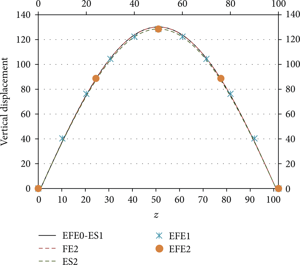
Plot of the displacement field $\mathrm{\hspace{0.17em}\hspace{0.17em}}\stackrel{.}{v}\mathrm{\hspace{0.17em}\hspace{0.17em}}$ for the nonlocal material constant e₀ = 33.3 with n = 10 elements (EFE1), n = 4 elements (EFE2), and exact solution (ES2). The plot of the local solution is EFE0 (e₀ = 0) and the plot of the exact solution is ES1. The classical beam FEM with n = 50 elements is plotted in FE2.

In particular, the EFE analysis with e₀ = 0 provides the classical local solution (EFE0). Assuming e₀ = 33.3, the results of the EFE analysis with n = 10 and n = 4 elements are, respectively, labeled EFE1 and EFE2 in Figure 2. The nonlocal solutions EFE0, EFE1, and EFE2 can thus be compared with the corresponding exact solutions obtained by the resolution of the sixth-order differential equation which are plotted in ES1 for e₀ = 0 and in ES2 for e₀ = 33.3 (see Figure 2).

Figure 3 reports a close-up of the displacement fields evaluated in Figure 2 in the interval 40 nm ≤ z ≤ 60 nm which clearly shows the difference between the local and nonlocal EFE solutions.

Figure 3:

Close-up of the local and nonlocal displacement fields reported in Figure 2 in the interval 40 nm ≤ z ≤ 60 nm.

It is worth noting that the EFE solution with only 4 elements exactly matches the corresponding analytical solution. Further, the evaluated displacements with the EFE mesh composed of 4 and 10 elements, see Figures 2 and 3, clearly show that no mesh dependence or boundary effects are pointed out by the considered nonlocal EFE model.

Moreover, the FE solution obtained with the classical beam FEM considering a mesh composed of 50 elements is also reported in Figures 2 and 3. The associated displacement field is plotted in FE2 and the poor performance of this element is apparent since the nonlocal effect is not exhibited.

The plot of the displacement field $\mathrm{\hspace{0.17em}\hspace{0.17em}}\stackrel{.}{v}\mathrm{\hspace{0.17em}\hspace{0.17em}}$ for the value e₀ = 166.7 of the nonlocal material parameter is reported in Figure 4.

Figure 4:

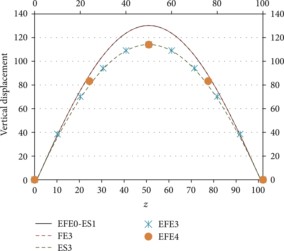
Plot of the displacement field $\mathrm{\hspace{0.17em}\hspace{0.17em}}\stackrel{.}{v}\mathrm{\hspace{0.17em}\hspace{0.17em}}$ for the nonlocal material constant e₀ = 166.7 with n = 10 elements (EFE3), n = 4 elements (EFE4), exact solution (ES3). The plot of the local solution is EFE0 (e₀ = 0) and the plot of the exact local solution is ES1. The classical beam FEM with n = 50 elements is plotted in FE2.

The results of the EFE analysis with n = 10 and n = 4 elements are labelled EFE3 and EFE4, respectively. As before, the EFE analysis with e₀ = 0 provides the classical local solution (EFE0). The nonlocal EFE solution is thus compared with the corresponding exact solution obtained by the resolution of the sixth-order differential equation which is plotted in ES1 for e₀ = 0 and in ES3 for e₀ = 166.7. A more significant nonlocal effect is apparent with increasing the nonlocal material parameter.

Moreover, Figure 5 reports a close-up of the displacement field plotted in Figure 4 in the interval 40 nm ≤ z ≤ 60 nm.

Figure 5:

Close-up of the local and nonlocal displacement fields in the interval 40 nm ≤ z ≤ 60 nm reported in Figure 4.

Also in this case, the nonlocal EFE solution with n = 4 elements best fits the exact solution and the results reported in Figures 4 and 5 with n = 4 and n = 10 elements clearly show that no mesh dependence or boundary effects are pointed out by the considered EFE.

For the considered nanobeam, the bending moment associated with the local and nonlocal models coincides as shown in Figure 6 where the plot ES is related to the exact solutions obtained by the sixth-order differential equation and EFE0, EFE1, and EFE2 denote the nonlocal enhanced finite element solution for e₀ = {0,33.3,166.7}, respectively.

Figure 6:

Plot of the bending moment: exact solution (ES), EFE0 with e₀ = 0 and n = 4 elements, EFE1 with e₀ = 33.3 and n = 4 elements, and EFE2 with e₀ = 166.7 and n = 4 elements.

5. Concluding Remarks

A thermodynamic analysis is developed in order to consistently derive a nonlocal finite element model for nanobeams. The adopted procedure is quite general and can be straightforwardly extended to different models of elastic nanobeams or to two-dimensional nanoelements.

A nanobeam under a uniformly distributed transverse load is considered. The numerical solution is obtained by the recourse to the proposed nonlocal enhanced finite element (EFE) procedure and the method shows no pathological behaviours such as mesh dependence, numerical instability, or boundary effects. A mesh composed of only n = 4 elements of equal size provides the exact solution in terms of displacement and bending moment thus showing the good performance of the proposed finite element method.