A Framework for Robust Address Assignment in WSNs Whispering to Avoid Intruders

Abstract

Wireless sensor networks (WSNs) are becoming bigger, and with this growth comes the need for new automatic mechanisms for initializations done by hand. One of those mechanisms is the assignment of addresses to nodes. Several solutions were already proposed for mobile ad hoc networks but they either (i) do not scale well for WSN; (ii) have no energy constraints; (iii) have no security considerations; (iv) or have no mechanisms to handle fusion of network partitions. We proposed an address self-assignment protocol which uses negative acknowledgements and an improved version of a flood control mechanism to minimize the energy spent; uses a technique named whispering to achieve robustness against malicious nodes; is able to detect dynamic network re-joint and dynamic node addition without exchanging specific messages; and handles both dynamic events without compromising routing tables.

1. Introduction

Wireless sensor networks (WSNs) have been arousing the interest of both researchers and the general community. WSNs are networks composed of small and cheap devices with sensing abilities which are able to communicate with each other through radio signals. The combination of sensing and radio communication abilities makes these networks ideal to build distributed sensing networks where each node collaborates by sensing one or more phenomena in its neighborhood and relaying it to a central node.

In order to be cheap and last for long periods without management, sensor nodes have several challenging constraints, from which the most important one is energy. Thus, every algorithm and protocol designed for sensor networks should always be energy conservative.

Given that sensor networks should be deployed on every kind of environment, including very hostile environments, security should be a major concern. Usually, achieving security implies some energy loss. However, this loss should be kept to a minimum when there is no threat to defend against.

1.1. The Naming Problem

One of the problems of sensor networks is the naming. Given that a sensor network could be comprised of a large amount of nodes, the unique addressing of each node may be a problem. Currently, nodes are initialized by hand with a unique number when the code is uploaded to the sensor node. In the initial versions of wireless sensors’ operating systems, every sensor had to be programmed individually through physical contact using a special programming device. In those days, initialization was not a big issue because it could be easily done with the programming. However, currently, wireless sensors are being programmed using their wireless network [1, 2], which makes naming much more difficult.

Given that sensor programming is currently done by wireless radio and that wireless radio communications require addressing each individual sensor, the naming cannot be piggybacked on sensor programming as it used to be.

The 6LowPan [3] initiative solves this problem by assigning an IPv6 address to each node, which ensures its uniqueness because it results from the combination of the personal area network (PAN) address, where the node is, and the 64 bit unique manufacturer address of the node's link layer [4]. Since these data are known by each node, the assignment can be done without contacting the neighborhood, thus achieving a zero configuration solution. However, 6LowPan assumes the existence of a link layer address and depends on its existence. 6LowPan is specially tuned to be used with the 802.4.15 link layer which supports two types of address: a 64 bit address and a 16 bit address. The 64 bit address is a global unique manufacturer address, and the 16 bit address is a dynamic address unique only within each PAN. The 16 bit address is used whenever possible because 64 bit addresses make the communication headers too big for small devices. In TinyOS, the usual payload length is 29 bytes, and the maximum packet size in 802.15.4 radio is 128 bytes [5]; thus, it is very inefficient to use 16 bytes just for the link layer addressing purposes (8 bytes for the receiver and 8 for the sender).

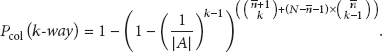
The 802.15.4 [6] 64 bit unique address is manufacturer specified; thus, it is always available, but the 16 bit address must be derived by a special protocol that ensures its uniqueness within the PAN. Notice that it is not possible to use the random assignment solution, as in IPv6 self-assigned addresses, because the probability of two nodes choosing the same address (a.k.a address collision) is given by the birthday paradox $p(X(n_t))=\mathrm{1}-{\prod }_{i=\mathrm{1}}^{n_t-\mathrm{1}}‍(\mathrm{1}-i/{\mathrm{2}}^{\mathrm{16}})$ , in which X is a discrete uniform distribution of addresses and $n_t$ is the total number of nodes deployed. As it can be seen in Figure 1, the collision probability is over 10% with only 120 nodes and reaches 50% with ~300 nodes.

Figure 1

Collision probability with the number of nodes deployed.

The 802.15.4 link layer address assignment protocol (LLAA) assumes the existence of a single PAN coordinator. The coordinator is responsible for defining the address domain to be used with the PAN and for dividing that address domain between its direct neighbors. Each of the neighbors takes one address for itself and divides the remaining addresses by its direct neighbors. The protocol continues until every node has an address. This protocol clearly does not scale well; it is prone to waste of address space if the tree created during the assignment is not balanced; it does not handle well node hording; and it is easily attacked by a malicious node near the coordinator; for example, it may take every address for itself, thus preventing others from getting addresses.

Besides LLAA, several other proposals have been made to dynamically assign short unique addresses to nodes [7–14]; however, most assume that every node in the PAN must have a unique address [7–9, 11] and/or that there is one central coordinator for each PAN [10, 12–14]. While the latter assumption is mostly true, although not always, the former requirement is often unnecessary.

Addresses are necessary both for identification and routing; however, both global identification and routing are often done with other types of identifiers. Often, the only requirement is that the addresses are locally unique, that is, that only the direct neighbors of each node have distinct addresses [15, 16].

In WSNs, nodes are often identified by data attributes and not by their unique global addresses. For instance, in the direct diffusion protocol [17], communication is data centric. A node requests data by sending an interest to named data. This interest is propagated to its neighbors, building an interest tree. Whenever a source needs to send data, the data flows hop by hop over that interest tree to all nodes that have manifest interest in it. In this situation, there is no need for a global node identification, since only data must be named, although local addresses are still needed to exchange messages between neighbors.

On the other hand, 6LowPan drafts define two types of routing: “mesh-under” and “route-over” routing [4]. The former usually requires PAN unique addresses, unless some sort of direct diffusion routing protocol is used, but the latter only requires local-unique MAC addresses, because the actual routing is done with IPv6 addresses. In this case, the MAC addresses are used to distinguish the message source and destination within the same “network segment,” that is, within the radio range of the source node, because every node behaves as an IPv6 router. There are several reasons to prefer “route-over” to “mesh-under” routing, the main one is that every existing network diagnostic tool for IP management will not work if a “mesh-under” routing is used [18].

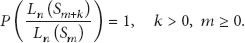
Assuming that only local unique addresses are needed, the problem is much more simple, but we still cannot use random self-assigned addresses, because the probability that k nodes, in the direct vicinity of each other, choose the same address over an address space of size $|A|$ , on a network with N nodes and an average of $\bar{n}$ neighbors per node, is given by (1)

$$\begin{array}{cc}& P_{\text{col}}\left(k\text{-}way\right)=\mathrm{1}-{\left(\mathrm{1}-{\left(\frac{\mathrm{1}}{\left|A\right|}\right)}^{k-\mathrm{1}}\right)}^{\left(\begin{array}{c}\left(\begin{array}{c}\bar{n}+\mathrm{1}\\ k\end{array}\right)+\left(N-\bar{n}-\mathrm{1}\right)\times \left(\begin{array}{c}\bar{n}\\ k-\mathrm{1}\end{array}\right)\end{array}\right)}.\end{array}$$

(1)

As it can be seen in Figure 2, the number of nodes that need to be deployed to have a 10% collision probability with an average of 20 neighbors, with an address space of 16 bit, is just 356.

Figure 2

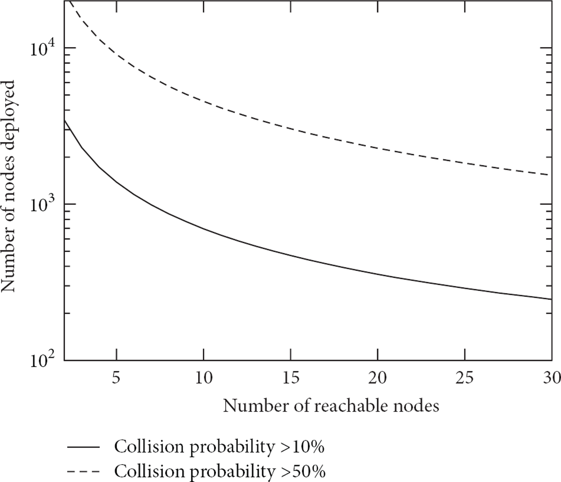
Number of nodes deployed for achieving a 10% and 50% collision probability with the average number of nodes directly reachable by each node.

1.2. Proposal

We have developed a message efficient and secure protocol to ensure the distribution of local unique addresses among neighbor nodes. The protocol is more efficient in terms of number of messages than similar ones, and it is secure against a bounded number of malicious nodes and is able to handle late deployment scenarios and partition rejoining without resetting established addresses (i.e, without breaking established routes between nodes).

The protocol efficiency is obtained through the use of only negative acknowledgements and through an improvement over a previously proposed flooding control technique. The security features of the protocol are obtained without cryptography, through a technique named whispering. We are assuming that sensor nodes are sold without key material in place. If cryptographic keys are going to be needed, they will be distributed later over the wireless medium together with sensor programming. Finally, the solution to handle partition rejoining is accomplished using nicknames between sensors.

The next section describes relevant related work. Sections 3 and 4 describe and evaluate the basic protocol and the solution to avoid intruders, respectively. Section 5 describes the solution to handle the incremental deployment of new sensors, and, finally, Section 6 concludes and presents future work.

2. Related Work

The naming problem which we intend to solve has been addressed before for WSNs and for mobile ad hoc networks (MANET). The IETF Zeroconf working group proposed a solution for MANETs [7] that rely on the discovering abilities of the underlying routing protocol. In this proposal, each node independently chooses an address and then sends a routing requesting packet to that address. If a route is found within a timeout period, it concludes that the address is already in use; otherwise, the address is not used and the protocol ends. The main problem of this protocol is the definition of the timeout when the number of hops needed to reach every node in the network increases. The protocol was developed for MANETs and does not scale well for WSNs where the number of nodes and hops between them is much higher.

Unlike the Zeroconf working group proposal, most naming solutions’ goal is to find a unique 2-hop address. This problem is known as the neighborhood unique naming (NUN) problem and is similar to the classical coloring graph problem with conditions at distance 2. In [19], it is proven that there is no determinist self-stabilizing algorithm to solve the NUN problem in uniform and anonymous networks under a distributed scheduler, and it proposes a self-stabilizing probabilistic algorithm. The algorithm is very simple: each node keeps two variables, one with its address and one with the address of two colliding nodes in its neighborhood; if there are no collisions in the neighborhood, the second variable is empty; each node starts by asking every neighbor their address to calculate the second variable; it then asks its neighbors for their variables’ values; if any of these values is equal to its own address, the node randomly chooses another. The algorithm was proven to self-stabilize, although no protocol was given to implement it. In particular, it is not clear how messages from two distinct nodes with the same address can not be confused with a repetition of a previous message.

The same strategy is followed in [20], but instead of using the 2-hop neighborhood, it uses a 3-hop neighborhood and a cache in every node to keep the addresses of its 3-hop neighborhood. It claim, that by using the 3-hop neighborhood it bounds each node number of attempts to choose an address. However, no consistency protocol for the 3-hop neighborhood cache is given, which makes it difficult to calculate the average number of messages required to reach a consistent state.

A cache is also used in [15] to keep addresses of direct neighbors. In this proposal, each node sends a periodical message with its address. This message is stored in the cache of its neighbors. If a node detects that two of its neighbors have the same address, it sends a warning message to one of them. With this protocol, nodes may change addresses several times during the lifetime of the network which may not be acceptable by every application or routing protocol. Moreover, the periodic broadcasting of addresses may be too energy expensive, and the authors fail to prove the self-stabilization of the protocol.

The approach followed in [8, 9] is different but also probabilistic. They leverage on the wireless nodes’ ability to detect media access collisions to know if there are other nodes contending for an address or not. If a node discovers that no one else is broadcasting at the same time, it takes the address for itself, and everyone else knows that that address is taken. If several nodes broadcast at the same time, they all flip a coin to decide if they will participate in the next round. On average, only half of the contenders transmit in the next round. After several rounds, only one node will transmit and will get the address. Although simple, this solution assumes that the radio is able to listen at the same time it transmits, which is not true in most inexpensive radio transmitters.

The solution proposed in [15] is able to handle dynamic scenarios by periodically repeating the protocol. In this proposal, each node sends a periodical message with its address. Each node keeps a log with every message seen by it; if it detects a duplicate address, it sends a warning message to both nodes. Upon receiving the warning message, both nodes choose another address and announce it again. With this protocol, nodes may change address several times during the life-time of the network which may not be acceptable by every application or routing protocol. Moreover, the periodic broadcasting of IDs may be too energy expensive, and it is not clear how the periodic address announcement is not mistaken with an address collision.

The work of [11] proposes the use of the location of each node in space to assign a unique field address but does not describe how to run a localization protocol without addresses or how to cope with common localization errors produced by such protocols.

With the exception of the solution described in [21], most 2-distance graph coloring algorithms and address assignment protocols are either deterministic and semicentralized or distributed and probabilistic. The reason why distributed protocols are probabilistic is the fact that, under a distributed and unfair scheduler, every node may precisely copy all the other nodes’ movements always choosing the same addresses; thus, the algorithm may never end. Clearly, a deterministic solution is better than a probabilistic one, because there is always the possibility that it never ends. However, most deterministic solutions do not scale well because they are either centralized or semi-centralized.

The centralized solution is never used in MANETs or WSNs. It would be similar to having a DHCP server replying to every node, which clearly does not scale beyond a few dozens of nodes. The semi-centralized solutions work by starting the assignment process at one specific central node and then distributing the assignment workload among other nodes. The DRCP and DAAP protocols [10] work together to assign addresses in MANETs. The DRCP is used by the node requesting an address as in DHCP: the node starts by asking if any of its neighbors is acting as a DRCP server, and if some of them reply, it chooses one of them to get the address from. After having received the address, the node uses the DAAP protocol to ask its DRCP server for half of its pool of addresses, and it then proceeds by acting as a DRCP server.

As described before, the 802.15.4 protocol uses two types of addresses: 64 bit global unique addresses and 16 bit network unique short addresses. The 64 bit addresses are used at the beginning of the network deployment to establish the 16-bit addresses, which are used thereafter. The protocol which establishes the 16-bit addresses is similar to DRCP/DAAP. However, instead of using two distinct steps for assigning an address and for assigning a pool of addresses, 802.15.4 only uses one; instead of giving up half of its address space to each child node, a node equally divides its pool of addresses among its neighbors.

The 802.15.4 distribution of addresses is specially unfitted for very unbalanced field topologies. This problem is handled in [12] by adapting the address distribution strategy to the network topology, at the cost of some more messages. The work of [13] also tackles the same problem but chooses a different solution. Although centralized, the proposed protocol does not define the addresses centrally; instead, it uses the relative hop-count location of each node to the other nodes to build each node address. The central node is used just as the center of a radial coordinate system, which is built by exchanging messages with that central node.

Another centralized protocol is proposed in [14]. Although the goal of the protocol is the establishment of a field unique address, it starts by specifying a local unique address to allow for point to point communication in the rest of the protocol. However, the description of this first phase is very short, and it advocates that a simpler beacon system is enough to detect address collisions within the protocol, which is not true because the address must be unique in a 2-hop scenario and not only in a 1-hop scenario.

None of the centralized or semi-centralized address assignment protocols scale well when the number of nodes is too large or the address space is too small. The solution presented in [21] does not have this problem, but it is costly in terms of time. In essence, the solution uses a token to establish an order between nodes’ address assignment, which in a network of several hundred nodes may take some time. Moreover, this solution requires the synchronized update of state variables in both sender and receiver nodes. This is a problem when nodes do not have a valid address, because in such situations, it is difficult to establish a single receiver.

Finally, most 2-distance graph coloring algorithms [21–23] try to find the graph coloring which uses the minimum number of colors. We have a much more relaxed goal. We want to find a 2-distance graph coloring with a minimum number of messages, bounded by a maximum of ${\mathrm{2}}^{\mathrm{16}}$ colors.

3. Basic Protocol

The basic protocol objective is twofold: (i) ensure a unique local identification on the WSN over a distance 2 neighborhood with an arbitrary large probability $p<\mathrm{1}$ and (ii) minimize the energy loss by minimizing the number of messages sent and received.

The protocol assumes no local or global knowledge of topological information. This includes global and relative geographic coordinates, number of neighbors, local and global density, or even the global number of nodes. This is important in a scenario where most sensor nodes do not have a GPS module and are distributed randomly over the sensor field. In such scenario, it is not possible to know geographic information at every sensor without running a localization protocol, which can only be run if proper addressing is in place. Therefore, although topological information may be acquired in the future, it is not available at initialization time.

Unlike several initialization protocols [19, 20], we have chosen to keep state variables private to each node; that is, we avoid the use of caches with partial knowledge of the state variables of other nodes. Although such caches would improve the nodes’ knowledge over their neighborhood, we avoid expensive cache coherence protocols.

The basic protocol is very simple, each node chooses a random address for itself and asks its neighbors if they have chosen the same address. If at least one of them has chosen the same address, it replies with a NACK, saying that a collision was found; otherwise, each receiving node rebroadcasts the query to its own neighborhood. The nodes receiving these rebroadcasts check the receiving packet for a collision with their own addresses. If they find a collision, they reply in the same way as the first hop nodes does; otherwise, they do nothing. A complete description of the protocol is given in Listings 1, 2 and 3. Listing 1 contains the main functions, the init() function initiates the address assignment protocol of each node, and the receive() function handles the reception of every message from the protocol.

Listing 1: Main protocol functions. The init() and receive() functions are the main protocol functions.

typedef enum {

 Query, NACK, ColQuery, ColReply, ColSolve} msgtype_t;           // Message Types.

typedef struct  {                           // Message structure.

 uint16_t   d_add,   s_add;                      // Destination and source addresses.

 msgtype_t   type;                          // Message type.

 byte   hop;                             // First or second hop.

 uint64_t   xadd  $[\mathit{4}]$ ;                           // Vector with extend addresses.

} msg_t;

uint16_t   myAdd;                         // Assigned short address

uint16_t   queryPower,   replyPower;               // Query and Reply transmission power variables.

uint16_t   pwrStep                // Power step reduction.

uint64_t   myXAdd,   prev_xadd;             // Extended address and previous extended address.

Name: init

Description: Starts the address self-assignment procedure.

init() {

 myXAdd= largerandom();                          // Choose a random extend address

 queryPower = replyPower= MaxPower;              // Sets the power step

 pwrStep = (MaxPower − MinPower)/NCircles;            // for each ring

 newAddress();                      // Chooses a new address

}

Name: receiveMsg

Description: Processes each received message. The “Query” and “NACK” message types are part of the address

     assignment protocol, while the “ColQuery”and “ColReply” are part of the collision solving protocol.

void receiveMsg(message_t   msg) {

 switch(msg.type) {

 case Query:                    // Query message received

  if(msg.s_add== myAdd  &&  msg.xadd $[\mathit{0}]$ != myXAdd) { // Test if there is a collision

   sendNack(msg);                     // Send a NACK if there is a collision

  } else if(!duplicate(msg)){              // Test if a copy was previously received.

    if( msg.hop == 0) {                  // If it is a fist hop query schedule

     msg.hop = 1;                    // a message for transmission after some time.

      sendQueryAfter(msg,   delayStep*msg . strength/pwrStep)

    }

  } else if(incCtr(msg)>  MaxCtr)             // Inc. and test the $n^o$ of copies

     markAsTrans(msg);              // If bigger than threshold, remove

  break;                            // the message from the sending queue.

 case NACK:                          // Negative ACK received

  if (msg.hop==1  &&                // If it is a NACK to a 2nd hop query

   (msg.xadd $[\mathit{1}]$ == myXAdd   ∣∣   msg.xadd $[\mathit{1}]$ == prev_xadd)) {  // that was sent by me

   msg.hop = 0;   sendNack(msg);            // Then send a NACK to the original query node.

  }

  if (msg.xadd[msg.hop]== myXAdd)           // If is is a NACK to a query sent by me

   if(add2Ctr (msg.hop)   ∣∣               // Inc. the counter of NACKs and if exceeds the

    (msg.hop==0 && msg.s_id== myAdd))             // threshold or I'm the original query node (1st hop),

     newAdd();               // choose a different address.

  break;

 case ColQuery:                  // Receive a Collision Query message

  msg ={msg.s_add,  myAdd,  ColReply,  myXAdd};         // Send a reply

  send(msg,  replyPower);              // with my short and extended addresses.

  break;

 case ColReply:                          // Receive a Collision Reply message

  if(isNotMsgScheduledTo(msg.s_add,   msg.xadd $[\mathit{0}]$ ))   $\{$          // if is the first message

   msg ={msg.s_add,  myadd,  ColSolve,  msg.xadd $[\mathit{0}]\}$ ;      // Schedule a ColSolve msg

   scheduleMsgToSend(msg,  timeout);           // with only its address

   falsePositives++;                // If no more ColReplies arrive this is a false positive

  } else {                    // If is the second message it confirms the collision

   addXAddToMsg(msg.s_add, msg.xadd $[\mathit{0}]$ ); // Add the extended address to the msg

   markAdd(msg.s_add);         // Mark the address as a collision

   falsePositives −−;              // Confirm that it was not a false positive

  }

  break; $\}\}$

Listing 2: Detecting an address collision using previous information on signal strength.

typedef struct {              // Node signal strength record

 uint_16 add;              // the address of this record

 byte ss_avg  $[\mathit{2}]$ ;           // signal strength average.

 byte n  $[\mathit{2}]$ ;               // messages received.

 boolean solving;           // is already solving a collision

} NodeRecord;

const int   maxMsgCount = 15;

Name: recMsgPwr

Description: Record the message strength for each source address and type.

      Analyses the previous maxMsgCount measurements and decide to start a collision solving procedure.

void recMsgPwr(int add,            // Source address

  int isB,                 // 1-broadcast, 0-otherwise.

  int ss) {             // signal strength.

 NodeRecord   nrec = getAddRecord(add);     // Find the record of the node with that address

 if (nrec.solving)                 // If its already solving a collision for the node

  return;                      // with that address, returns.

 if(nrec.n[isB] >)0 {             // If the number of messages record for that address is >0

  int  ci = 4 + falsePositives;            // Set the confidence level to 4 (4*sigma: −99.99% ci) plus

                        // the number of false positives to dynamically adjust the ci.

  byte diff = abs(ss  −  nrec.ss_avg[isB]);   // Diff between the signal strength (ss) and the average ss

  if(diff > ci*0.003*ss)          // If diff is bigger then the confidence level

    startColSolving(add);               // starts the collision solving protocol

 }

 if(nrec.n[isB] > maxMsgCount) {              // If the number of record msgs is bigger then the maximum

  nrec.n[isB] = 1;                  // resets the count and

  nrec.ss_avg[isB] = ss;                  // the signal strength average

 } else {

  nrec.n[isB]++;                  // Increments the message record count

  int delta = ss  −  nrec.ss_avg[isB];         // calculates the new signal strength

  nrec.ss_avg[isB] += delta/nrec.n[isB];   // average.

 }

}

Listing 3: Auxiliar functions.

Name: newAddress

Description: Generate a new short address and send it after a random delay

 

void newAddress() {

 myAdd = random();                // Generate a new random short ID.

 sendQueryAfter(msg,   randDelay);            // Sends a Query for that short ID.

}

Name: add2Counter

Description: Counts 1st and 2nd hop NACKs and reduces transmission power accordingly

boolean add2Counter(byte hop) {             // Count the number of NACKs received.

 static int secCtr

 secCtr += hop==0?1:3;              // A NACK at the 2nd hop decreases power faster than at 1st.

 if (secCtr>9  &&  queryPower>0)  $\{$             // If to many NACKs were received:

  queryPower−= pwrStep;                // decreases the power, unless power

  secCtr = 0;              // is already zero; resets the counter;

  prev_xadd = myXAdd;              // saves the previous extended address;

  myXAdd= largerandom();                // and generates a new one.

  return true;                     // Inform that a new short address must

 }                           // be generated.

 return false;                 // There is no need to generate

}                            // a new short address yet.

void sendQueryAfter(msg_t msg, int delay)  {       // Query messages are sent

 msg.type = Query;

 msg.xadd[msg.hop] = myXAdd;          // with the extended addresses

 sendAt(msg,   queryPower, time()+delay);          // and with current queryPower.

}

void sendNack(msg_t msg) {

 msg.type = NACK; send(msg,  replyPower);        // NACK messages are sent

}                          // with replypower.

Notice that there are no positive replies, only negative ones. This is because the probability of finding a node with the same address in a 2-hop neighborhood is very low; thus, in the usual scenario, only query messages are sent. Note that the probability that a node in a 2-hop neighborhood chooses the same address of the query node is given by $p_c(|A|,\bar{n})=\mathrm{1}-(\mathrm{1}-\mathrm{1}/|A|{)}^{\mathrm{4}\bar{n}}$ , that is, ~ $\mathrm{1}{\mathrm{0}}^{-\mathrm{3}}$ for a 20 node neighborhood and a 16-bit address space, which is much lower than the probability of finding a collision in a 2-hop neighborhood (the birthday paradox).

The first problem that the protocol needs to overcome is how to distinguish the rebroadcast messages originated in itself from the ones originated in other sensors. If a node trying to establish an address receives a query for that same address, it should answer declaring that that address has been taken, even if that action results in neither of the nodes sticking with the address. However, if the node is hearing an echo of its own query, it should do nothing. Thus, we need a way to uniquely identify the messages.

The messages sent by each node are stamped with a collision free 64 bit node address (extended address). This extended address can be a manufacturer unique number, when available, or a random number generated whenever a node starts. However, as we will describe later, a random number is preferred over a manufacturer unique number for security reasons. Note that extended addresses are only used in the context of the initialization protocol. Afterwards, only short addresses are used. In fact, the protocol can be seen as a recoloring protocol with a smaller color space.

Two other similar problems happen when a rebroadcast node needs to relay a NACK back to the original querying node and when a node receives a NACK for its own address. In both cases, nodes should only act upon NACKs which were triggered by their own queries; otherwise, the protocol may not stabilize.

Self-stabilization, as defined in [24], is an important property of a distributed protocol. It ensures that regardless of the initial state of the system and regardless of the scheduling of actions taken by each participating node the system will reach a legitimate final state in a finite number of steps.

Beauquier et al. [25] redefined self-stabilization for probabilistic protocols in such a way that regardless of the initial state of the system and regardless of the scheduler strategy the system will reach a legitimate final state with probability 1. Using the framework for proving self-stabilization of probabilistic protocols defined in [25], it can be shown that the previously described protocol, satisfies the above mentioned definition of self-stabilization, if extended addresses are used to link queries and replies.

Informally, the framework, defined in [25], states that a probabilistic protocol is self-stabilizing for a given specification if there is a sequence of predicates over system states $L_i(S_k)\cdots L_n(S_k)$ where $S_k$ is the system state at step $k\ge \mathrm{0}$ and $n>i\ge \mathrm{0}$ such that the following conditions hold.

• (i)

  The last predicate $L_n(S_k)$ (known as the legitimate predicate) of the sequence is a predicate that identifies a legitimate final state according to the specification.

• (ii)

  For every scheduler, the probability of reaching a system state satisfying the specification from a state verifying the legitimate predicate is 1, which can be formalized by the following conditional probability:

  $$\begin{array}{cc}& P\left(\frac{L_n\left(S_{m+k}\right)}{L_n\left(S_m\right)}\right)=\mathrm{1},\hspace{1em}k>\mathrm{0},\hspace{0.17em}\hspace{0.17em}m\ge \mathrm{0}.\end{array}$$

  (2)

• (iii)

  For every scheduler strategy, if the probability of reaching a state verifying one predicate in the sequence is 1, then the probability of reaching a state verifying the next predicate in the sequence is also 1, which can be formalized by the following conditional probability.

  $$\begin{array}{cc}& P\left(\frac{L_{i+\mathrm{1}}\left(S_{m+k}\right)}{L_i\left(S_m\right)}\right)=\mathrm{1},\hspace{1em}k\ge \mathrm{1}.\end{array}$$

  (3)

The first two are easily verified by the protocol. If we choose n to be the total number of nodes, and $L_i(S_k)=\{N_{\text{cf}}(S_k)⩾i\}$ , where $N_{\text{cf}}(S_k)$ is the number of nodes with a collision free address in state $S_k$ , the last predicate ( $L_n(S_k)$ ) clearly identifies a legitimate final state (first requirement). Moreover, after reaching a legitimate state (i.e. every node has a 2-hop unique identifier), the protocol ceases to send NACKs. Since addresses are only changed when a NACK arrives, the system will reach a final configuration verifying the specification (second requirement).

To prove that the protocol satisfies the last requirement, we will use another result from [25]. It states that the third requisite is verified if predicates are closed and verify the local convergence property. A predicate $L_i$ is closed if for every $S_k$ and $m>\mathrm{0}$ , $L_i(S_k)\Rightarrow L_i(S_{k+m})$ . Two predicates are said to verify the local convergence property if, according to a scheduling strategy, the probability of reaching a state verifying the second predicate from a state verifying the first predicate, in less than $k>\mathrm{1}$ steps, is greater than $\delta >\mathrm{0}$ .

The predicate $L_i(S_k)=\{N_{\text{cf}}(S_k)⩾i\}$ is closed under the given protocol, because whenever a node chooses a 2-hop unique address and every 2-hop neighbor has the opportunity to reply and does not do it, the node sticks with that address forever, provided that it only acts upon NACKs to its own queries. Notice that, if the node tries to optimize the process of detecting a collision by overhearing NACKs to queries initiated by other nodes, it does not verify this property and may not stabilize.

Given the collision probability $p_c$ and the probability of finding a 2-hop unique identifier $p_s=\mathrm{1}-p_c$ , the probability of collision after k independent trials is $P_c(k)=p_c^k$ , and the probability of success is $P_s(k)=\mathrm{1}-p_c^k$ . Thus, if we take $\delta =P_s(k-\mathrm{1})$ , then $P_s(k)>\delta$ , provided that $p_c<\mathrm{1}$ . Notice that after only three trials the collision probability is in the order of magnitude of ~ $\mathrm{1}{\mathrm{0}}^{-\mathrm{10}}$ for networks with a neighborhood density from 8 to 16 nodes and a 16 bit address space.

3.1. Broadcast Problems

One of the previously described problems of the protocol is that it relies on broadcast messages. Broadcast messages are inherently unreliable because whenever the number of nodes in the neighborhood is not known, the emitter will not be able to know if messages have arrived or not. However, in WSNs, the problem is even worse because messages may not arrive for many more reasons than in other network scenarios:

• (i)

  the well known hidden terminal problem in radio networks may prevent messages from arriving without being noticed by the emitter;

• (ii)

  depending on the MAC protocol, nodes may have the receiver asleep, to prevent energy loss, when a broadcast message arrives.

The common solution to improve broadcast reliability is to repeat each broadcast message several times to improve the probability of being received. However, this solution increases the potential of message collision whenever several nodes are trying to broadcast a message. When some of these messages are rebroadcasts of previously arrived broadcast messages, we may be faced with the so called broadcast storm problem [26].

To reduce the broadcast storm problem, we use the counter-based solution proposed in [26] enriched with distance information. In the original counter-based solution, some nodes are prevented from rebroadcasting a received message in order to minimize the number of messages sent. Whenever a node receives several replicas of the same message, it concludes that most of its neighbors have already received the message; thus, it does not need to send it again. By avoiding sending messages, nodes are minimizing the broadcast storm problem and are saving energy, but they are increasing the probability of not reaching nodes that they should. In [26], it is shown that, in a homogenous radio network, the uncovered area of a rebroadcast is directly related to the number of copies already received. In the original implementation, nodes rebroadcast after a random delay, provided that in the meantime they have not received enough copies of the same message. In the proposed solution, nodes further away from the source broadcast first, thus increasing the probability that nodes closer to the source are prevented from broadcasting.

There are other methods to minimize broadcast storms with better efficiency ratios, that is, the ratio; between the covered area and the number of broadcasting nodes is better with other methods. However, all these methods require either the knowledge of the topological localization of each node [26] or, at least, each node's neighbors [27].

In the proposed protocol, after receiving a query message, the node checks if that message has been previously received. If the message has been previously received more than a specified number of times, the message is marked as transmitted. Otherwise the message is scheduled for broadcast after a delay directly proportional to the power of the received message (line 44 in Listing 1). The result is that the retransmission area is divided into concentric rings. The nodes in each of these rings rebroadcast at more or less the same time. Notice that rings are not evenly distributed in space because the reception power varies with the inverse square of the radius, which is more or less consistent with the error in measuring message strength, which is much bigger for low power receptions; that is, outer rings are wider than inner rings because outer nodes have less accurate positioning than inner nodes.

The first question that arises is the number of copies that need to be received in order to prevent the message to be rebroadcasted. Williams and Camp [28] found that for networks with densities lower than 11 neighbors this threshold must be ≥4 to get a maximum coverage, that is, minimize the number of nodes that never receive the message. However, their scenario is different from ours (we need to cover a 2-hop region while they need to cover the whole network), and they do not use the reception signal strength to schedule rebroadcasts.

We have modified the 802.11 MAC layer of the J-Sim simulator [29] to incorporate our identity assignment features and tested over a field of $n=\mathrm{300}$ nodes using the free propagation model. The sensors were placed randomly on a rectangular field with an area $A=(n/(k+\mathrm{1}))\pi r^{\mathrm{2}}$ , where r is the maximum transmission distance and $k=\mathrm{12}$ is the average number of neighbors of a node. The results are depicted in Figures 3, 4, 5, 6, and 7 and are analysed below.

Figure 3

Impact of the threshold value on the percentage of messages not delivered, with and without power aware rebroadcast delay.

Figure 4

Energy spent by each node (divided by the energy spent by a single message transmission) for a given coverage.

Figure 5

Number of messages sent by node with threshold value and density.

Figure 6

Impact of whispering over the percentage of affected nodes, in the presence of a percentage of badly behaved ones.

Figure 7

Relation between the percentage of failed nodes with the percentage of malicious nodes and network density, with and without whispering.

The graph in Figure 3 shows the impact on the percentage of uncovered area with the chosen threshold. As expected, the uncovered area decreases when the threshold increases. However, it can be seen that the threshold required to achieve a significant coverage is much lower with the signal strength information than without it. To get a coverage of 99.5% (i.e., 0.5% of messages not received), we need a threshold of 6 without reception power information and a threshold of 4 with reception power information.

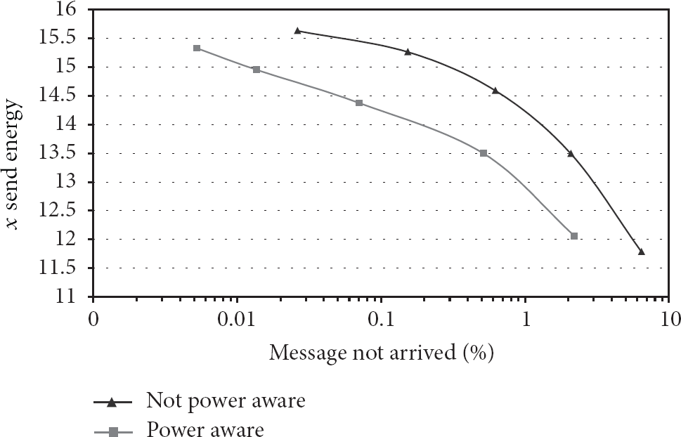
A lower threshold is better because it reduces the number of messages sent, thus improving energy consumption and minimizing the broadcast storm problem. In the end, the choice is between energy and coverage. Figure 4 shows the energy spent by each node as a function of the desired coverage. In this graph, we have assumed a simplified energy model in which sending a message consumes one energy unit, the reception of a message consumes $\mathrm{1}/\mathrm{10}$ of a unit, and everything else is negligible.

Again, as expected, the coverage increases with energy consumption both in the original solution and in the improved one. However, the solution which makes use of reception strength information is able to achieve better coverage with the same energy. In some cases, the uncovered area is 10 times smaller with the same energy consumption.

The resulting protocol is very fast. Figure 5 shows that each node sends around 4 to 12 messages on average to ensure the completeness of the protocol depending on the density of the field (threshold values have very little effect).

However, it is clear that even with this model some of the messages are not going to be delivered which may affect the correctness and stability of the protocol. It is obvious that the stability of the protocol is not affected because the number of NACK messages does not increase. On the other hand, the correctness is clearly affected because if a query or a NACK message does not reach some of the neighbors, two or more nodes may choose the same address without noticing. However, the probability of an undetected collision is very small (for a 99.5% coverage, the probability of a 2-way undetected collision on a network with 1000 nodes and 20 neighbors is ~0.1%) and may be handled by the protocol described in Section 5.

4. Avoiding Intruders

The previous scenario assumes that every node behaves well. If one or several nodes start replying to every query saying that they have already chosen that address, the well behaved nodes may end up with a depleted battery after repeating the query several times. If well behaved nodes do not share individual cryptographic key material with every neighbor, they are not able to distinguish well behaved neighbors from badly behaved neighbors. In such scenario, the only solution is to speak progressively softly until the badly behaved nodes are not able to hear the query. This is similar to whispering to your neighbor to prevent intruders from overhearing.

Whispering prevents nodes from communicating with more distant nodes which may have a negative impact on the network connectivity. We minimize this impact by reducing the power only as much as necessary and only in the nodes which are direct neighbors of the badly behaved one. Notice that, if a node receives a NACK originated at his neighbor's neighbor, reducing the power may prevent it from communicating with legitimate neighbors which are closer to it than the badly behaved node. It is its neighbor that should reduce transmission power. However, a node can not know for sure if a NACK is being relayed or produced at its neighbor, since a badly behaved node may always forge a NACK as if it were being relayed. Our solution was to reduce the power more quickly at nodes receiving NACKs to be relayed. Therefore, the only way a malicious node is able to force another node to reduce its transmission power rapidly is by being near; otherwise, it can only affect the node through relayed NACKs.

The reduction of transmission power should only affect queries, and the reply messages should be transmitted at full power; otherwise, a node could be prevented from sending a NACK only because it has a badly behaved node near it (see line 55 of Listing 1 and function add2ctr() in Listing 3).

After receiving a query from a node, a badly behaved node may start issuing NACKs to random addresses, even if it does not receive any more queries (because of query power reduction) trying to guess the next chosen address. To prevent it, a node should change its extended address every time it reduces its query transmission power.

A final word about the necessity of keeping the previous extended address after changing to a new one: the previous extended address is required whenever a node changes its address and it was already participating in another query as a relay node. If a NACK arrives, it must be relayed because there is no way to tell if that is a legitimate NACK from a colliding node or a malicious one.

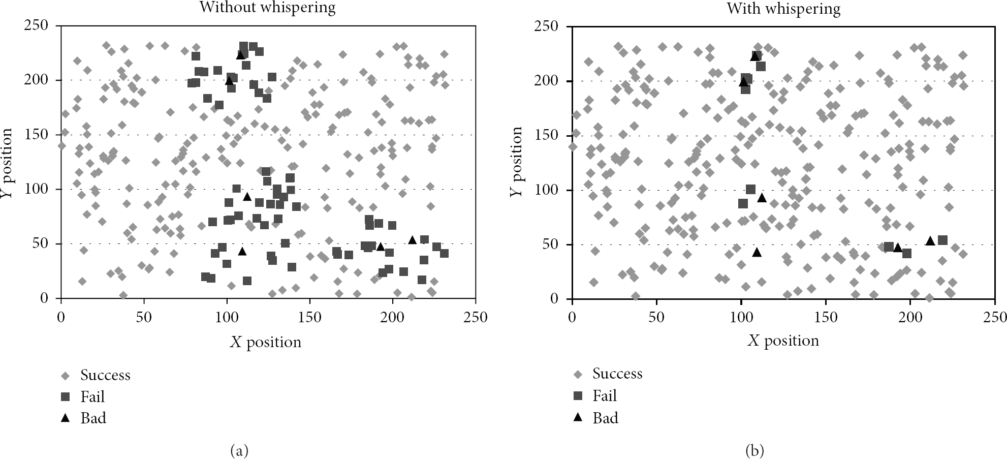
This protocol is not able to completely prevent badly behaved nodes from stopping well behaved ones from choosing an address, but it minimizes the number of affected nodes. We have tested it by modifying a small percentage of nodes of our J-SIM simulator such that they behaved as malicious nodes would, if they wanted to prevent the protocol from succeed. We assumed that malicious nodes are also energy constrained and are not able to be radiating messages all the time. Instead, they reply with NACK messages to every query and continue to do so for a period after receiving the query, trying to guess the extended address used by the request that is whispering. As before, the number of nodes was set to 300 and the wireless range and deployment field size was chosen such that the average number of neighbors of each node is $k=12$ .

Figure 6 shows the effect of a small percentage of malicious nodes (2%) over a field of 300 randomly deployed nodes. Dark triangles represent malicious nodes, light rhombus represent nodes that were able to choose a collision free address, and dark squares represent nodes that were not able to choose an address or became isolated from nonmalicious nodes by the effect of power reduction.

As expected, the number of nodes which were not able to get an address with whispering is much smaller than without it. With whispering, the affected nodes are in the direct vicinity of the malicious nodes, while without whispering, the affected nodes are spread over their 2-hop neighborhood.

The number of affected nodes is obviously dependent on the number of badly behaved ones, but it is also dependent on the network density. The number of failed nodes increases when the number of nodes in the vicinity of malicious ones increases. Figure 7 shows how the percentage of affected nodes increases with the percentage of malicious ones and with the network density. In both cases, the percentage of failed nodes is much lower and increases much slower with whispering than without whispering. In fact, with whispering, the variation of failed nodes with the network density is almost negligible, while without whispering, the effect is very noticeable.

5. Handling Incrementally Deployed Scenarios

One important feature of address assignment protocols, which is often forgotten, is its ability to handle late deployed sensors and merging of network partitions. The deployment of additional sensors may be necessary either to improve the sensor coverage or to improve the network lifetime; the sensors in place may be at the end of its battery. The merging of network partitions may happen either because there was an obstacle dividing nodes at the time of deployment which is now removed or because the addition of new nodes made two or more networks reachable to each other.

In such scenarios, address collisions may happen, because at the time of address assignment, not every node knew about each other. Most address assignment protocols do not consider these scenarios, and the ones that do choose to rerun the assignment protocol in the colliding nodes [15]. This strategy may have a negative impact on routing, because every route established through those nodes needs to be rebuilt.

Another problem that these protocols need to handle is how to detect the existence of colliding addresses. In [15], address collisions are detected during the periodically neighborhood query which is done for this purpose. However, given that the addition of new nodes and the merging of networks are rare, such a scheme is too energy expensive. In [30] (a protocol designed for MANETs), each packet has an additional 64 bit unique number which is used to detected address collisions, but that is not an option in WSNs given the size of each packet.

Whenever a node is added or a barrier is lifted between two or more network partitions, it is possible that two or more nodes with the same address became reachable by a single node. A k-way collision happens whenever k nodes with the same address are reachable by one node, a.k.a the detecter. The probability of having a k-way collision after the address assignment protocol runs is given by the probability of having a k-way collision $P_{\text{col}}(k\text{-}way)$ (1) times the probability of a k-way cut during the address assignment protocol. Assuming that a 2-way cut is given by $p_{\text{cut}}(\mathrm{2}\text{-}way)$ , then the probability of a k-way cut is given by

$$\begin{array}{cc}& p_{\text{cut}}\left(k\text{-}way\right)={\left(p_{\text{cut}}\left(\mathrm{2}\text{-}way\right)\right)}^{\left(\begin{array}{c}k\\ 2\end{array}\right)},\end{array}$$

(4)

because it requires a cut between every two pairs of nodes in the k-way collision.

Figure 8 shows the probability of collision for 3-way and 2-way collisions for several number of nodes after running the address assignment protocol, giving an address space $|A|={\mathrm{2}}^{\mathrm{15}}$ (15 bit addresses, we will use the extra bit for collision solving), a neighborhood of 25 nodes, and a probability of a 2-way cut of 1. The collision probability is around $\mathrm{1}{\mathrm{0}}^{\mathrm{7}}$ times below for 3-way collisions in comparison with 2-way collisions.

Figure 8

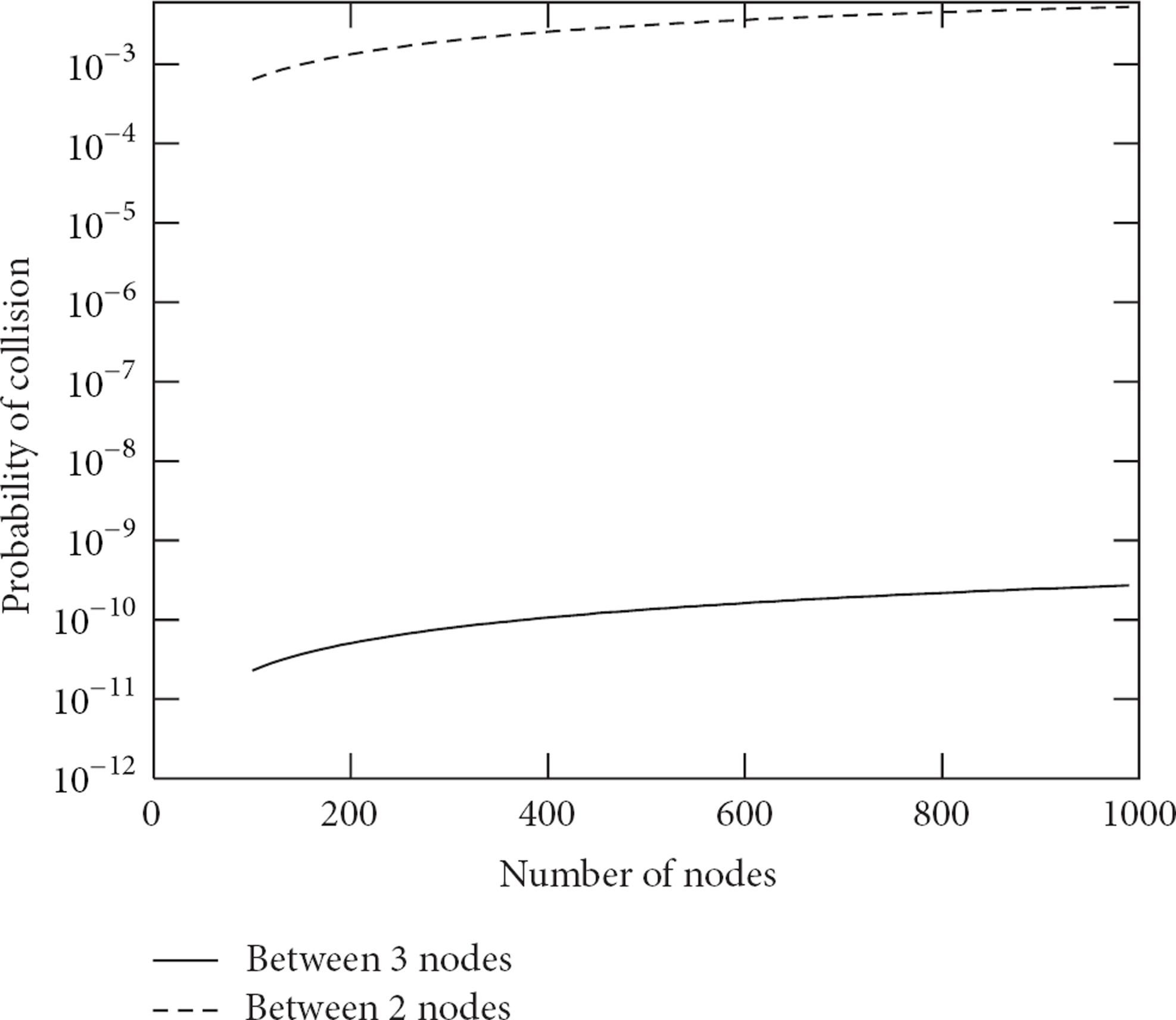
Collision probability between 2 nodes and between 3 nodes for a field with a density of 25 neighbors.

Given the above results, we make the hypothesis that k-way collisions with $k>\mathrm{2}$ are extremely unlikely, and we are going to focus our efforts in detecting and solving 2-way collisions.

5.1. Detecting Address Collisions

Our approach to detect address collisions is motivated by the way that people distinguish two voices in a crowd. If one of the voices is loud and the other is soft, then there are probably two persons talking. If the heard sentences do not make sense because they seem garbled, then it is possible that they are produced by more than one person. Neither of these heuristics gives precise information about the existence of colliding addresses, but they may be used as triggers for a collision solving protocol.

The former solution is independent on the transport protocol, while the latter is not. In order to detect out-of-order messages, the transport protocol must have the notion of order which is not the case for many transport protocols in WSNs; this is why we have chosen the former solution.

Given the hypothesis that only 2-way collisions may happen whenever the network changes, only two scenarios are possible:

• (i)

  the address of the added node is the same of one of the nodes already in the network, and both are reachable by a third node (merge of partitions),

• (ii)

  the address of two of the nodes in the network is the same, and they are reachable by the new node (node addition).

The first scenario is simpler than the second, although, as we will see, they will be handled the same way. If the nodes in the network knew each other, they are able to know the signal strength (SS) average and standard deviation of messages sent by each other. If one of the nodes detects a message with a SS much different from the usual, it may suspect an address collision, although, to be sure, it will have to run the collision solving protocol described in the next section. The second scenario is a bit more troubling because the colliding nodes are both new for the detecting node.

We have started by using an algorithm from Knuth [31] to incrementally calculate the average $\overline{\text{SS}}$ and standard deviation ${\sigma }_{\text{SS}}$ of the SS without having to keep all samples, that is, the calculus is incremental. In order to get a four nines confidence level in the collision detection, we checked if the SS of each message was within four times the standard deviation of the average (5):

$$\begin{array}{cc}& \left|\overline{\text{SS}}-\text{S}{\text{S}}_i\right|<\mathrm{4}{\sigma }_{\text{SS}}.\end{array}$$

(5)

Otherwise; we would signal a collision. However, we have realized that the SS average varies over time due to battery drain and environment changes, leading to large standard deviations and making the system irresponsive to address collisions. Figure 9 shows a typical signal strength over time of messages received in a field of MicaZ Motes using the TinyOS 802.15.4 stack; the measurements were taken between two sensors 1 meter apart sending a message to each other, every second, for 150 seconds long. The first approach to solve this problem was to calculate the SS average and standard deviation using only the last few messages; however, that too proved ineffective because the standard deviation with too few messages lacked the necessary precision.

Figure 9

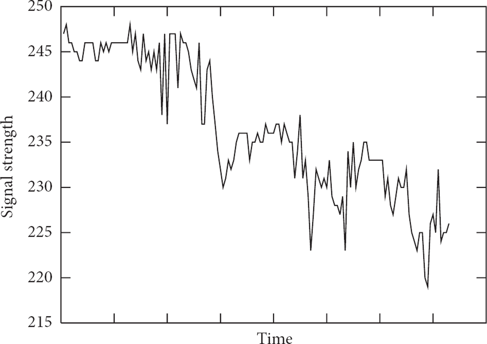
Signal strength of messages received by the same node over time.

Instead of computing both the average and standard deviation, we chose to compute the average over the last few messages and estimate the standard deviation based on the average. In order to do it, we have analyzed the standard deviation of messages’ SS sent by the same node at different distances and in different places.

We have realized that the most relevant factor to the measurements of standard deviation is the place where the measurements were done, in particular if the test site has many wifi antennas working. This is consistent with several reports of interference between Wifi and 802.15.4 networks. We called such scenarios noisy ones and all the others nonnoisy since we did not find other relevant differences.

Figure 10 depicts the standard deviation variation with signal strength and noisy versus non-noisy environments. We have placed two nodes transmitting at 1, 5, 10, and 15 metters in noisy and non-noisy environments and measured the average and standard deviation of the received signal strength for each distance and environment over 150 messages. For each calculated average, we have plotted the correspondent standard deviation and drawn a line showing that, frequently, standard deviation is higher for higher reception strengths. As expected, the standard deviation over a few messages is very small in low noise scenarios and is almost twice in high noise scenarios (Figure 10).

Figure 10

Standard deviation behavior with the signal strength ( $\text{S}{\text{S}}_{\max }=\mathrm{255}$ ) of messages.

A good compromise is given in Figure 10, in which the predicted standard deviation is given by ${\widehat{\sigma }}_{\text{SS}}=\mathrm{0.003}\text{S}{\text{S}}_i$ . Our measurements showed that (5) with ${\widehat{\sigma }}_{\text{SS}}$ instead of ${\sigma }_{\text{SS}}$ is suitable both for low and high noise scenarios; however, if for extremely high noise scenarios the number of false collisions detected by this protocol is too high, we incorporate a self-regulatory mechanism which increases the standard deviation every time a false positive is detected.

This solution has another advantage: it is able to handle both collision scenarios. Notice that, if a node arrives to a network and starts to communicate with two other nodes with the same address at the same time, it will not have previous information about average and standard deviation; therefore, it will not be able to find discrepancies with past history. However, with this solution, although the average will still be wrongly calculated because it will be something in between the two signals of the two communicating nodes, the standard deviation will not change much, which will allow the detection of the collision.

Listing 2 shows that whenever a message is received with a signal strength above or below a predefined confidence interval the solving protocol (see Section 5.2) is started. Notice that the set of values kept for each address is comprised by: the average of the signal strength of every message received (ss_avg); the number of messages received from that address; and a value indicating that a conflict is being solved. Notice, also, that the record structure uses two sets of values for each address, because it is expected that broadcast communications be done with a different transmission power than unicast communications. The transmission power of unicast communications is usually adapted to the distance between peer nodes, while the broadcast communications do not have this kind of adaptation.

We have conducted two sets of experiments, using MicaZ sensor nodes running TinyOS 2.0, in three different environments: two small non-noisy environments and one open and noisy environment, that is, a large student hall with many students moving, each one with its own laptop device with Wifi and many Wifi antennas in the vicinity. The first set of experiments was designed to detect false positives, and the second to detect false negatives.

5.1.1. False Positives

The false positive ratio is an important metric because it impacts the energy consumed by each node in the collision solving protocol; that is, running the collision solving protocol is expensive and should be triggered as seldom as possible. We have placed two nodes at different distances (1, 5, 10, and 15 meters) sending messages to each other and measured the amount of times that the algorithm detected a false collision (Table 1), that is, the number of times one of the nodes received two messages from a single node, with signal strengths different enough to be mistakenly identified as coming from two different nodes with the same ID. We have conducted 10 experiments at each distance and environment, each experiment exchanging 300 messages (150 messages each), and we have taken the average number of false positives. As expected, the number of false positives in the non-noisy scenarios was close to 0% which is consistent with the four nines accuracy specification. In the noisy environment, the system showed a rate of almost 11% of false positives without the regulatory mechanism, but with the regulatory mechanism, after just 3 false positives, it reached a steady state where no more false positives occurred (0% false positives).

Table 1

Error rate at different distances (in meters) and noise levels.

False detections	Regulatory mechanism	Noisy environment					Nonnoisy
		1 m	5 m	10 m	15 m	Total	total
Negatives		0%	1%	3%	0%	4%	0%
Positives	Without	6%	1%	0%	4%	11%	0%
	With	0%	0%	0%	0%	0%	0%

Another interesting result is the distribution of false positives with the distance. Most false positives (6%) were experienced when the colliding nodes were 1 meter apart from the arriving node. For larger distances, within the transmission ratio of our nodes (in noisy environments 15 meters), the false positive rate is much lower, which may be related to the saturation of the signal (it is difficult to distinguish two persons shouting very near to us).

5.1.2. False Negatives

Although we have defined two collision scenarios: the arriving node connecting two networks previously disconnected and the arriving node having the same address of another node, we have only measured the false negatives in the former, because it is more general than the latter. The main difference between the two scenarios is the node that detects the collision; in the “connecting two networks scenario” it is the arriving node that detects the collision while in the “arriving node scenario with duplicate address” it is one of the other existing nodes that detects the collision. From a detection point of view the main difference between the two detecting nodes is that the former one has no history of messages received (it has just arrived) and the latter may have received messages before from one of the duplicate address nodes. Therefore the former scenario is harder to detect. Moreover, the algorithm specifies that after a predefined number of messages (maxMsgCount) the history of received messages is cleaned, therefore in the long run the two scenarios are equal.

In order to assess the false negative rate of the first scenario, we have chosen the worst possible placement of nodes for the purpose of collision detection. Assuming that all nodes have an equal radio range, the arriving one will be in the position of connecting two previously disconnected nodes with potentially the same address if it is placed within the intersection of the two radio coverages, and the difficulty of detecting the collision will be higher when the node is placed at the exact same distance of the two colliding nodes (Figure 11), since it will receive messages from both of them with similar strength. Again, we have conducted 10 experiments with 150 messages each at each combination of distance, environment, and regulatory mechanism (with and without) and taken the average number of times that the collision was not detected.

Figure 11

Area where the arriving node needs to be placed in order to detect the collision. The dark rhombus represents the arriving node and the light circles the colliding nodes.

The protocol shows 0% of false negatives (Table 1) if it is closer to one of the colliding nodes or if it is run in a low noise environment; however, in a high noise environment with the two colliding nodes at exactly the same distance, we have experienced a false negative rate of 4%. A false negative does not mean that the arriving node will never detect the collision, it just means that it is not able to detect the collision within the frame period of 2 times maxMsgCount. Nonetheless, fast detection is important to minimize the impact of garbled communications.

5.2. Collision Solving Protocol

The collision detection protocol described in the previous section does not provide a definitive answer on the existence of an address collision. It ends by sending a query to every node with a specific address. Only if several nodes reply (with different extend addresses) the collision is confirmed.

When a node detects a collision, it gives to every node with the same address a nickname, and informs the node of that nickname The situation is similar to having two students in the same class named John, and we refer to one as “Little John” and to the other as “Big John.” Notice that they will still be named John for every one else, and we cannot just name them “Little” and “Big,” because we would create other collisions.

The solution is to reserve one bit from the 16 bit addresses for nicknames. Therefore, only 15 bit of the 16 bit addresses are assigned by the address assignment protocol, and the remaining bit is originally set to zero. When a node detects a collision it informs each of the colliding nodes that one of their addresses will have to set the bit to one. Each of the colliding nodes stores in a table the nickname for which it is known by that node. Whenever the node that changed its address receives a message from the node that detected the collision, it will only accept it if the bit on the destination address is set to one. Notice that other nodes continue to communicate with the node that changed the address with the old address; the change is only relevant for the communication with nodes that detect the collision.

This solution is only able to solve a single collision. If the address of a node collides with two other nodes, the protocol does not work because it would be possible for a node to end up being known by two nicknames by two different nodes, which would have a negative impact in broadcast communications. In fact, unicast communications would not be affected because the node could choose the nickname to use depending on the message destination; however, for broadcast communications, the node would not know the nickname to choose. Nevertheless, this is not a big problem because 3-way collisions are much less probable than 2-way collisions.

The proposed algorithm is shown in Listing 1. The algorithm assumes that the node detecting the collision (the initiator) has sent a “collision query” message (ColQuery) to all the nodes with the colliding address (line 26 in Listing 2). After receiving that message, a node replies with its extended address. When the initiator receives a “collision reply” (ColReply) message, it schedules a “collision solving” message (ColSolve) to be sent after a predefined timeout. If the node receives another “collision reply” message with a different extended address, it confirms the existence of a collision. If that happens, it marks the address that has a collision and modifies the “collision solving” message waiting to be sent by adding the new extended address. Finally, upon receiving the “collision solving” message, the colliding nodes choose independently the one that is going to adopt a nickname by comparing the extended addresses. The one with the smallest extended address adds a nickname to its address. Note that whenever there is no collision, that is, the collision detection protocol had a false positive none of the nodes adopts a nickname, because the smallest extended address in the message is 0 which is an invalid extended address.

The cleanMsg function is used whenever a message is received. If the message comes from someone with a nickname and the receiver has not detected that collision (some other node did), the nickname bit is clean. This ensures that a node that adopted a nickname may use it in broadcast communications.

6. Conclusion

The address self-assigning problem is a well-studied problem in the MANET world, but it has not received much attention in the WSN world. In this paper, we have described a simple address self-assignment protocol and proved its correctness. To improve the protocol performance, we have proposed an improvement to a well-known method of controlling message floods, based on the level of the power of message reception.

We have introduced the whispering technique to handle intruders when cryptographic keys are not available or have been compromised and show how to use it in the proposed protocol. We believe that this is a valid security technique and intend to study its application in other protocols.

We have designed and tested a very energy efficient mechanism (it does not use specific messages for that purpose) to detect late address collisions with a very low error rate. Finally, we have proposed the use of aliases to handle late address collisions without disrupting routing and other session tables.

The combination of all these protocols result in a very robust address assignment framework which was implemented in TinyOS 2.0 and tested in MicaZ motes.