Location Algorithm for Nodes of Ship-Borne Wireless Sensor Networks

Abstract

Node location is of great significance as a supporting technology of wireless sensor network (WSN). The information without position would be greatly devalued. So this paper is about location algorithm for nodes of ship-borne WSN based on research on structure of ship and work environment of ship-borne WSN. The whole location process consists of two steps: one is location algorithm among cabins (LAAC), and the other one is location algorithm in the cabin (LAIC). LAAC refers to location with the topology of ship-borne WSN. We can learn which cabin the node lies in. LAIC refers to location based on received signal strength indication (RSSI), we can get distance relationship between nodes by RSSI, and then obtain the specific location by solving this distance relationship. In the last part, this paper verifies the designed location algorithm by experimenting on “A” ship. Experiments show that the location algorithm designed by this paper is feasible.

1. Introduction

Although WSN has been widely used in many fields, the study of ship-borne WSN is still in its infancy. At present, the research for ship-borne WSN mainly contains two aspects: first, some researchers have studied the communication of WSN on shipboard [1, 2]; second, some researchers have proposed the idea of using WSN to monitor work environment on shipboard [3–5]. For example, some researchers use WSN to monitor the temperature of the engine room.

To improve the safety of navigation and achieve the goal of early warning, we have proposed another application of WSN that is monitoring the environment and the state of cargo on shipboard, especially the dangerous cargo. Due to loading, unloading of cargo, and changing of equipments, the position of ship-borne WSN nodes is indeterminate. If crew cannot attain the position of nodes, emergency measures would be delayed in case of an alarm, so to save time in taking emergency measures, it is necessary to get the position of WSN nodes; that is to say, we should design location algorithm for ship-borne WSN and find out which cabin the node lies in and the specific position within the cabin.

So far, there have been many WSN location algorithms, among which location algorithms based on RSSI [6, 7], time of arrival (TOA), angle of arrival (AOA), and distance vector-hop (DV-hop) [8, 9] are most popular. RSSI is a measurement of the power present in a received radio signal, which would decrease with the increase of distance between the sender and the receiver. Compared with other ranging methods, it is more convenient to acquire RSSI, and we do not need to add any hardware device. For example, RSSI can be easily read from the 8-bit RSSI. RSSI_VAL register of the RF module CC2420 [7].

The WSN has different performances in different application environments, and location algorithm is related to the application environment of WSN. Ship-borne WSN has its own characteristics compared with the traditional WSN. For example, the spatial distribution of ship-borne WSN nodes is three dimensional, the variability of topology is confined, and the nodes on different decks cannot communicate directly. The detail of these characteristics would be introduced in the next part. Due to the characteristics of ship-borne WSN, the existing algorithm is not very suitable for ship-borne WSN. And, as we know, there is not any location algorithm for ship-borne WSN. In addition, the location of WSN node is very important for the safety of the ship. So it is necessary to make research on the location algorithm of ship-borne WSN.

2. Ship-Borne WSN

Ship-borne WSN consists of a large number of nodes, which can be divided into three categories based on the function of nodes. They are common nodes, repeaters, and base stations, respectively. The common node is responsible for collecting and transmitting data; the repeater is responsible for repeating the data which were transmitted to the base station by common nodes; and finally the base station is responsible for receiving the data from WSN and transmitting these data to the computer. Figure 1 shows the structure of ship-borne WSN. Compared with the traditional WSN, ship-borne WSN has its own characteristics.

Figure 1

The schematic diagram of ship-borne WSN.

The characteristics of ship-borne WSN are shown as follows.

(1)

The spatial distribution of ship-borne WSN nodes is three dimensional. There are many decks on ship, and many cabins on each deck. Unlike distribution of ship-borne WSN nodes, the distribution of traditional WSN nodes stays almost on the same panel. So the distribution of ship-borne WSN nodes varies greatly compared with the traditional WSN nodes.

(2)

The variability of topology is confined. A ship is constructed by joining many blocks together, and blocks are made of steel plates cut or welded, which means that the ship is a large structure made mainly of steel. This metallic structure shields radio signals. This will severely attenuate the transmitting of nodes. Compared with the traditional WSN, the variability of ship-borne WSN topology is confined.

(3)

The nodes on different decks cannot communicate directly. They mainly communicate through the repeaters located at the stairs between decks [10].

(4)

The nodes in the same cabin have similar route; that is to say, they would transmit data to the base station by the same repeater. It should be noted that “cabin” in this paper refers to the area in which the nodes have the similar route when they transmit data to the base station. That is to say, the division of cabins is related with the location of repeaters and the structure of the ship.

(5)

The nodes in the same cabin would construct a small sensor network which can be referred to as subnet, as shown in Figure 1.

With so many characteristics, it is indispensable to study ship-borne WSN and location algorithm.

3. Location Algorithm

To cope with the characteristics of ship-borne WSN, this paper has designed the location algorithm for nodes of ship-borne WSN. In the process of locating, we call the node, whose position is known, “anchor node” (AN) [11], and some anchor nodes should be prearranged in cabins before locating; we call the node waiting to be located “blind node” (BN) [12].

3.1. An Overview of Process of Location

The whole location process can be divided into two steps: the first is LAAC, and the second is LAIC.

First, we can acquire the name of cabin in which blind node is arranged, according to LAAC. And then let the blind node transmit data to the anchor nodes in the cabin and record the RSSI value. According to these RSSI values, we can build up the distance relationship between blind node and anchor nodes in the cabin. At last, we can calculate specific location by solving this distance relationship. Figure 2 shows the flow of location for ship-borne WSN. As can be seen from the figure, the location result consists of two parts: one is the name of the cabin, and the other one is the specific position in the cabin.

Figure 2

The flow diagram of location.

3.2. Location Algorithm among Cabins (LAAC)

LAAC refers to pinpointing the name of cabin in which the blind node locates by the route of packets received by the base station from the blind node. We can analyze these packets, construct the topology of ship-borne WSN, decide the route, and get the repeater nearest to the blind node. Finally, according to the repeater, we can get the name of cabin where the blind node is by looking up the relational table, which contains the IDs of repeaters and the names of cabins.

Figure 3 shows the flow of LAAC. First, we should arrange repeaters and record their positions. Because of the complicated structures of ships, it is necessary to arrange these repeaters properly. Two rules should be obeyed: one is to make sure that the ship-borne WSN can communicate normally; the other one is to try our best to let the blind nodes in one cabin transmit data to the base station by the same repeater. According to the characteristics of ship-borne WSN, repeaters should be arranged at stairs of decks. Then, we can make relational table by the location of repeaters. The table contains the ID of repeater and the name of cabin in which the blind node lies, which would transmit data to the base station by this repeater. The format of relational table is shown in Figure 3.

Figure 3

Location algorithm among cabins.

When the base station receives packets from the blind node, we can get the repeater nearest to the blind node by analyzing the route. At last, checking the relational table, we can get the name of the cabin in which the blind node lies.

The process of locating the algorithm among cabins is described as follows.

(1)

The base station acquires the route of packets from the blind node: $B_{r} = {$ BN, Repeater_1, Repeater_2, Repeater_N,…, Base station}.

(2)

Analyze the route and acquire the ID of the nearest repeater to the blind node, NR_B_ID.

(3)

Acquire location by the relational table: $S = {$ (Repeater_1_ID, cabin_number_1), (Repeater_2_ID, cabin_number_2),…, (Repeater_N_ID, cabin number_N)}.

(4)

According to the NR_B_ID, check the location by the relational table S and acquire the cabine_nuber_i.

(5)

Get the name of the cabin in which the blind node locates.

3.3. Location Algorithm in the Cabin (LAIC)

LAIC refers to geting the three-dimensional coordinates in the cabin according to RSSI values after confirming the cabin number in which the blind node lies.

In the cabin, there are some anchor nodes, which were arranged before location, and we can get the IDs and coordinates of these anchor nodes from the database. When we want to locate the blind node, we can let it transmit packets to these anchor nodes in the cabin, and then the anchor nodes are activated. In order to decide the signal transmission model, actually to decide the path loss exponent, these anchor nodes start to communicate with each other until the path loss exponent is decided. After the path loss exponent is decided, these anchor nodes just receive the packets from the blind nodes and transmit these RSSI values to the base station. RSSI is related with distance, so we can get the distance relationship between the blind node and these anchor nodes according to the path loss exponent. The following formula describes the relationship between RSSI and distance:

\begin{matrix} P_{r} (d) - P_{r} (d_{0}) = - 10 β \log (\frac{d}{d_{0}}) + X_{dB}, \end{matrix}

(1)

where X_dB is a zero-mean Gaussian random variable (in dB), β is the path loss exponent, and $P_{r} (d_{0})$ is the average of signal strength at a reference distance $d_{0}$ (1 m in our case) [13].

At last, we can calculate the specific coordinates of blind nodes using this distance relationship. The flow of LAIC is shown in Figure 4.

Figure 4

Location algorithm in the cabin.

According to the analysis of LAIC, we can know that there are 3 types of packets transmitted in the process of location. The first category is the packets of location transmitted by the blind nodes, and we call them packet_A. The second category is the packets transmitted among anchor nodes to decide the signal transmission model, and we call them packet_B. And the last category is the packets which contain RSSI values, and we call them packet_C. The format of packets in LAIC is shown in Figure 5. ID_A indicates the ID of the sender, and ID_B is the ID of the receiver.

Figure 5

Three types of packets in LAIC.

Assume that there are N anchor nodes in the cabin and that the coordinates of ith anchor node are ( $x_{i}$ , $y_{i}$ , $z_{i}$ ); the coordinates of the blind nodes are (x, y, z), and the distance from the blind node to the ith anchor node is $d_{i}$ , so we can get the following formula:

\begin{matrix} {(x_{i} - x)}^{2} + {(y_{i} - y)}^{2} + {(z_{i} - z)}^{2} = {d_{i}}^{2}, \end{matrix}

(2)

where i is, respectively, $1, 2, 3, \dots, N$ . Due to the error of distance, we cannot solve formula (2). However, it is possible to estimate a position which is close to the real position, and we call this position the “estimated position.” In order to let the estimated position and the real position to be closer, we make the quadratic sum of difference value between the distance from the estimated position to anchor nodes and the measured distance minimum, which is the least square algorithm. So we have the following formula:

\begin{matrix} Δ d = \sum_{i = 1}^{n} W_{i} {(\sqrt{{(x - x_{i})}^{2} + {(y - y_{i})}^{2} + {(z - z_{i})}^{2}} - d_{i})}^{2}, \end{matrix}

(3)

where $Δ d$ is the quadratic sum of difference between the distance from the estimated position to anchor nodes and the measured distance, and $W_{i}$ is the weighed factor ( $1 / d_{i}$ in our case). That is to say, the estimated position ( $\hat{x}$ , $\hat{y}$ , $\hat{z}$ ) makes function $Δ d$ (x, y, z) minimum. At point ( $\hat{x}$ , $\hat{y}$ , $\hat{z}$ ), the partial derivation is zero, and the partial derivation is shown as in the following formula:

\begin{matrix} \frac{\partial Δ d (x, y, z)}{\partial x} = 0, \\ \frac{\partial Δ d (x, y, z)}{\partial y} = 0, \\ \frac{\partial Δ d (x, y, z)}{\partial z} = 0 . \end{matrix}

(4)

Solving these equations, we can get the estimated position [14].

For location algorithm based on range, the location error is influenced by distance errors and geometric errors, in which geometric errors refer to the errors caused by the spatial arrangement of blind node and anchor nodes when the distance errors are constant. Geometric dilution of precision (GDOP) can describe geometric error. GDOP is shown as in the following formula:

\begin{matrix} GDOP = \sqrt{\frac{σ_{x}^{2} + σ_{y}^{2} + σ_{z}^{2}}{σ^{2}},} \end{matrix}

(5)

where σ is the distance error and $σ_{x}$ , $σ_{y}$ , and $σ_{z}$ are the location errors in three directions. It is thus evident that geometric error is just related with spatial arrangement. The smaller the GDOP is, the smaller the geometric error is, and the better the spatial arrangement is, the bigger the GDOP is; the bigger the geometric error is, the worse the spatial arrangement is. It is proved that GDOP is inversely proportional to the volume of the shape constructed by unit vectors from the blind node to anchor nodes. The smaller the volume is, the bigger the GDOP is; the bigger the volume is, the smaller the GDOP is [15].

4. Experiments on Shipboard

In order to verify the location algorithm designed by this paper, we experimented on the “A” ship. The deckhouse of the “A” ship consists of the following decks: arranged vertically (from bottom to top): the tank top; tween deck; main deck which houses several classrooms; promenade deck; boat deck; captain deck; navigation deck; and compass deck. The eko node and the IRIS node produced by crossbow are used in the experiments. The radio frequency of ship-borne WSN is 2.4 GHz, the transmitter power output is 3 dBm, and the receive sensitivity is −101 dBm.

4.1. Experiments for LAAC

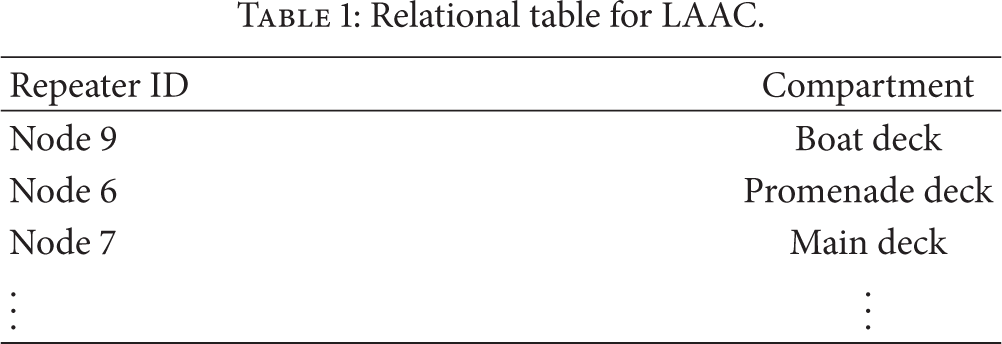
According to LAAC, we arrange the repeaters; the positions of repeaters are shown in Figure 6, and the relational table is made and shown in Table 1. After network, the topology of ship-borne WSN is shown in Figure 6.

Table 1

Relational table for LAAC.

Repeater ID	Compartment
Node 9	Boat deck
Node 6	Promenade deck
Node 7	Main deck
⋮	⋮

Figure 6

Topological structure of ship-borne WSN.

Assume that Node 4 is the blind node, by analyzing the received packets, we can acquire the route: Node 4 → Node 7 → Node 6 → Node 9 → Base 0; the black arrow in Figure 6 shows the route. Then, we can find the nearest repeater: Node 7 to Node 4. At last, by looking up the relational table, we know that the blind node is on the main deck. And Node 4 is actually at the classroom of the main deck. It is obvious that LAAC is feasible.

4.2. Experiments for LAIC

Before the experiments for LAIC, the RSSI values in different distances are measured. In Figure 7 a graph is shown for scattering every distance (1 m, 2 m, 4 m, 6 m, 8 m, 14 m, 20 m, and 26 m). And the straight line in the figure is the mean RSSI value.

Figure 7

Reading RSSI on CC2420.

The experiment for LAIC is preceded in a cabin on the main deck. The scale of the cabin is 12 m × 8 m × 3 m. Before location, we had arranged 6 IRIS nodes in the classroom as anchor nodes. In the experiment, we tested 40 times for a node located at point (5, 4, 2). And the location result is shown in Figure 8. In this figure, the green pentagram indicates the true position of the blind node; triangles indicate location results, in which the color indicates the location error (location error refers to the distance between the true position and the estimated position); the black balls indicate anchor nodes. In Figure 8, the 3D view and the projective view of location results are displayed.

Figure 8

Location results.

In the projective figures, the distribution of location results indicates the location error in this plane. And the bigger the area of the distribution is, the bigger the location error of this plane is. The relation of the location error in three planes is shown in the following formula:

\begin{matrix} E_{X - Y} < E_{X - Z} < E_{Y - Z}, \end{matrix}

(6)

where $E_{X - Y}$ , $E_{X - Z}$ , and $E_{Y - Z}$ are, respectively, the location errors in $X - Y$ , $X - Z$ , and $Y - Z$ planes. The distance error in three planes is almost the same as each other. So the difference of location error in the three planes is caused by spatial arrangement of the blind node and anchor nodes, which is geometric error. According to the above paragraphs, we know that geometric error is related with the volume of the shape constructed by unit vectors from the blind node to anchor nodes. Figure 9 shows these unit vectors and the projective figure of the shape. The relation of the area is shown in the following formula:

\begin{matrix} S_{X - Y} > S_{X - Z} > S_{Y - Z}, \end{matrix}

(7)

where $S_{X - Y}$ , $S_{X - Z}$ , and $S_{Y - Z}$ are, respectively, the areas of the shape constructed by unit vectors from the blind node to anchor nodes in $X - Y$ , $X - Z$ , and $Y - Z$ planes.

Figure 9

The shape constructed by vectors from blind node to anchor nodes.

According to formulas (6) and (7), we can reach the following conclusion: the geometric error in each plane is influenced by the projected area of shape constructed by the unit vectors from the blind node to anchor nodes. The bigger the projective area is, the smaller the geometric error is; on the contrary, the geometric error is bigger.

Therefore, when we arrange these anchors, the geometric error should be fully considered.

Figure 10 shows the location error of experiment for LAIC, whose mean value is 1.5 m and RMSE (root mean square error) is 0.35 m. And the location error which is smaller than 2.0 m is 87.5 percent.

Figure 10

The error of location results.

5. Conclusions

By analyzing the characteristics of ship-borne WSN, this paper has designed and verified location algorithm for nodes of ship-borne WSN, which consists of LAAC and LAIC, and to test the location algorithm, we experimented on the “A” ship. Experimental results show that we can get the name of the cabin in which the blind node is by LAAC, and we can get the specific position by LAIC. In the cabin of 12 m × 8 m × 3 m, the precision of location is about 1.5 m.

The location algorithm can provide the position for nodes of ship-borne WSN. In case of an emergency, the algorithm can help the crew to locate the position of causes without delay and provide safeguard for life and property at sea. In addition, the location algorithm designed by this paper can also be used in the similar situation, for example, when WSN is used to monitor the condition of cargo hold and container. The reason is that it has a similar topology to the ship-borne WSN.

Footnotes

Acknowledgments

This work was supported by the National Natural Science Foundation of China (61073134; 51179020), the study on optimal model and knowledge-based support algorithm for three-dimensional search and rescue at sea, the study on optimal route design for ship under the condition of wind navigation aid, the State 863 Projects (2011AA110201), the system of and the key equipment for the integrated bridge, and the Applied Fundamental Research Project of the Ministry of Transport of China (no. 2013329225290).

References

Paik

B.-G.

Cho

S.-R.

Park

B.-J.

Lee

Yun

J.-H.

Bae

B.-D.

Employment of wireless sensor networks for full-scale ship application

Embedded and Ubiquitous Computing 2007 48 8 113 122

Kdouh

Zaharia

Brousseau

El Zein

Grunfelder

ZigBee-based sensor network for shipboard environments

Proceedings of the 10th International Symposium on Signals, Circuits and Systems (ISSCS ′11)

July 2011

Iasi, Romania

229 232

2-s2.0-80052626464

10.1109/ISSCS.2011.5978701

Liu

The research for application of WSN in engine room

Shanghai Shipbuilding 2008 73 1 34 36

Wang

The MAC Protocol Optimization and Simulation of WSN in Ship 2010

Dalian, China

Dalian Maritime University

Xiao

Research and Design of Temperature Monitoring System for Ship Engine Room Based on WSN 2008

Dalian, China

Dalian Maritime University

Daiya

Ebenezer

Murty

S. A. V. S.

Raj

Experimental analysis of RSSI for distance and position estimation

Proceedings of the International Conference on Recent Trends in Information Technology (ICRTIT ′11)

June 2011

Chennai, India

1093 1098

2-s2.0-80052215396

10.1109/ICRTIT.2011.5972367

Benkič

Malajner

Planinšič

Čučej

Ž.

Using RSSI value for distance estimation in Wireless sensor networks based on ZigBee

Proceedings of the 15th International Conference on Systems, Signals and Image Processing (IWSSIP ′08)

June 2008

Bratislava, Slovakia

303 306

2-s2.0-52949111029

10.1109/IWSSIP.2008.4604427

Tian

Zhang

Liu

Sun

Wang

A RSSI-based DV-hop algorithm for wireless sensor networks

Proceedings of the International Conference on Wireless Communications, Networking and Mobile Computing (WiCOM ′07)

September 2007

Honolulu, Hawaii, USA

2555 2558

2-s2.0-38049083700

10.1109/WICOM.2007.636

Wang

Agrawal

D. P.

Range-free localization using expected hop progress in wireless sensor networks

IEEE Transactions on Parallel and Distributed Systems 2009 20 10 1540 1552

2-s2.0-70349088999

10.1109/TPDS.2008.239

10.

Kdouh

Brousseau

Zaharia

Grunfelder

El Zein

Applying ubiquitous wireless technologies for shipboard monitoring systems

Proceedings of the 14th International Symposium on Wireless Personal Multimedia Communications (WPMC ′11)

October 2011

Brest, France

1 5

2-s2.0-83655169819

11.

Zhang

An improved localization algorithm for wireless sensor network using a mobile anchor node

Proceedings of the Asia-Pacific Conference on Information Processing (APCIP ′09)

July 2009

Shenzhen, China

485 488

2-s2.0-70450169080

10.1109/APCIP.2009.255

12.

Wang

R.-R.

Zhang

Z.-Y.

Wang

J.-Z.

Xue

A.-K.

A new solutions for staff localization in chemical plant

Proceedings of the International Conference on System Science and Engineering (ICSSE ′11)

June 2011

Macao, China

503 508

2-s2.0-84860416800

10.1109/ICSSE.2011.5961955

13.

Che

RSSI-based positioning of wireless sensor network technology

Instrument Technique and Sensor 2010 26 10 82 84

14.

Xiao

Research for Location of WSN Nodes Based on Least-Square and SVR 2011

Ganzhou, China

Jiangxi University of Science and Technology

15.

Sharp

Guo

Y. J.

GDOP analysis for positioning system design

IEEE Transactions on Vehicular Technology 2009 58 7 3371 3382

2-s2.0-69549105982

10.1109/TVT.2009.2017270