Channel Estimation for Relay-Based M2M Two-Way Communications Using Expectation-Maximization

Abstract

The growing popularity of machine-to-machine (M2M) communications in wireless networks is driving the need to update the corresponding receiver technology based on the characteristics of M2M. In this paper, an expectation-maximization-based maximum likelihood cascaded channel estimation method is developed for relay-based M2M two-way communications. As the closed-form solution of maximum likelihood channel estimation does not exist, and the superimposed signal structure at the receiver is conducive to the expectation-maximization application, the expectation-maximization algorithm is utilized to provide the maximum likelihood solution in the presence of unobserved data through stable iterations. Even in the absence of the training sequence, the cascaded channel estimates are obtained through the expectation-maximization iterations. The Bayesian Cramér-Rao lower bounds are derived under random parameters for the channel estimation, and the simulation demonstrates the validity of the proposed studies.

1. Introduction

Machine-to-machine (M2M) communication is expected to be one of the major derivers of cellular networks [1, 2] and has become one of the focuses in 3GPP [3]. M2M technology allows machine devices to communicate directly with each other without human intervention, which has been attracting more and more interests for their wide applications in many popular wireless communication systems, such as mobile ad hoc networks [1–3]. Wireless M2M networks supporting M2M-enabled machine devices are pivotal to the success of M2M. Sensor nodes in wireless M2M networks could be connected by a wide range of wireless network technologies, for example, cellular networks.

Cooperation is crucial in wireless networks as it can greatly attribute to ensuring connectivity, reliability, and performance. Relaying is promising in a wide variety of network types for the cooperation purpose. According to the recent IEEE 802.16p proposals, a wireless M2M device may act as an aggregation point and communicate data packets on behalf of the other M2M devices, which may have a poor communication link to the network. Relay-based schemes have been proposed to improve the link reliability for devices with weak links [4–7].

As a basic model of the relay-based M2M two-way communications, the three-node cooperation model, which is also referred to as the two-way relay channel, where two source nodes exchange information via a relay node using amplify-and-forward (AF) or decode-and-forward (DF) strategy, has attracted a great deal of research interest because of its improved spectral efficiency [8–12]. AF relaying is more popular in practice because the relays only amplify and process the signal linearly before they retransmit it again and thus AF leads to low-complexity relay transceivers. A lot of research therein assumes perfect channel knowledge at the nodes, which is unpractical in wireless communications, so it is important to develop efficient channel estimation algorithms. Channel estimation for this communication scene has been studied in [13–18]. Specifically, in [13] the maximum-likelihood-based estimator, flat-fading channels were reported, and in [14, 15], the cascaded source-relay-source channels were estimated using block-based training under the assumption of time-invariant frequency-selective fading channels although the individual channels were also estimated using pilot-tone-based training in [14]. Different from [14, 15], where the relay only amplifies and forwards the received signal, the work in [16] allowed the relay to estimate the channel parameters and allocated the powers for these parameters. The channel estimation problem was extended to the multiple antennas scene at all the three nodes in [17], and an optimal method was proposed to design the training signals based on the mean-square-error (MSE) criterion. A blind channel estimation algorithm by applying a nonredundant linear precoding at both source nodes was proposed for the frequency-selective channels in [18].

The expectation-maximization (EM) algorithm is a general method for solving maximum likelihood estimation problems given incomplete data, and it consists of two iterative steps: the expectation step and the maximization step. These two steps are iterated until the estimated values converge [19, 20]. The EM-based maximum likelihood estimation for one-way relay channel has been investigated in [21–24], where different variables are treated as the missing data and iterative process is provided for the channel estimation. To the best of our knowledge, the EM estimation algorithm in two-way relay channels has not been investigated yet.

Since the received signal at the source node in the relay-based M2M two-way communications is a superimposed signal, which can be decomposed into two signal components with two unknown channel parameters, one is the self-interference signal, and the other is the desired signal from the other source node. Take the channel estimation at source node 1, for example, the two unknown parameters are source1-relay-source1 cascaded channel and source2-relay-source1 cascaded channel. The source1-relay-source1 channel is the unobserved data when estimating source2-relay-source1 channel, while the source2-relay-source1 channel is also the unobserved data when estimating source1-relay-source1 channel. Since the superimposed signal structure at the receiver is conducive to the application of the EM algorithm and the closed-form solution of maximum likelihood channel estimation does not exist for this relay-based M2M two-way communication, the EM algorithm is utilized to provide the maximum likelihood solution in the presence of unobserved data through stable iterations.

In this paper, we propose an EM-based channel estimation algorithm for relay-based M2M two-way communication to jointly estimate the two cascaded channels. The idea is to decompose the observed data into its signal components and then estimate the parameters of each signal component separately. In the EM algorithm, the received signal at the source node is treated as the incomplete data, and the set of the two signal components from the two source nodes is modeled as the complete data. Conditioned upon the incomplete observations, the channel estimation algorithm maximizes the expectation of log likelihood function defined over the complete data, by averaging over the unknown underlying parameters and using the current estimates of the cascaded channels without channel statistical information. The algorithm iterates back and forth, using the current channel parameter estimates to decompose the received signal better and thus increase the likelihood of the next channel parameter estimates. Even in the absence of training sequence, the cascaded channel estimates can still be obtained through the iterations between the E-step and M-step. The Bayesian Cramér-Rao lower bounds are derived under random parameters for cascaded channel estimation, and the validity of the proposed studies is verified by Monte Carlo simulations.

The rest of the paper is organized as follows. Section 2 describes the three-node model in relay-based M2M networks. Section 3 presents the EM-based cascaded channel estimation algorithms. Section 4 provides the Bayesian Cramér-Rao lower bounds of the cascaded channel estimation. Simulation results and conclusion are given in Sections 5 and 6, respectively.

2. System Model

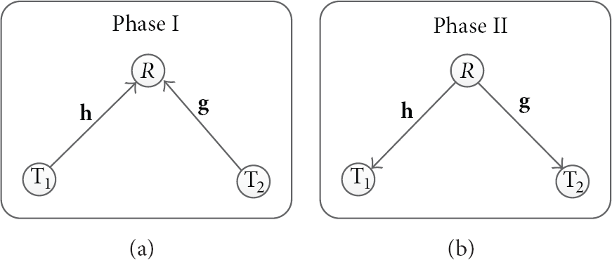
Consider a three-node cooperation model in wireless M2M networks where two source nodes, ${\text{T}}_{\mathrm{1}}$ and ${\text{T}}_{\mathrm{2}}$ , exchange information through one relay node R, as shown in Figure 1, which is also the model of two-way relay network. Each node has a single omnidirectional antenna and operates in half-duplex mode. The direct link between ${\text{T}}_{\mathrm{1}}$ and ${\text{T}}_{\mathrm{2}}$ is very weak or even nonexistent, and thus the source-destination communication is performed only via the relay. The transmission is divided into two phases. During Phase I, both ${\text{T}}_{\mathrm{1}}$ and ${\text{T}}_{\mathrm{2}}$ send a signal frame to R via an uplink manner, whereas during Phase II, R processes the received signals and broadcasts them to ${\text{T}}_{\mathrm{1}}$ and ${\text{T}}_{\mathrm{2}}$ .

Figure 1

Three-node cooperation model.

The baseband channel between ${\text{T}}_{\mathrm{1}}$ and R is denoted by $\mathit{h}={[h_{\mathrm{0}},h_{\mathrm{1}},\dots ,h_{L_h-\mathrm{1}}]}^T$ , and the one between ${\text{T}}_{\mathrm{2}}$ and R is denoted by $\mathit{g}={[g_{\mathrm{0}},g_{\mathrm{1}},\dots ,g_{L_g-\mathrm{1}}]}^T$ , where $L_h$ and $L_g$ are the numbers of the taps of the corresponding channel delay spread. $h_l\in 𝒞𝒩(\mathrm{0},{\sigma }_{h,l}^{\mathrm{2}})$ and $g_l\in 𝒞𝒩(\mathrm{0},{\sigma }_{g,l}^{\mathrm{2}})$ are independent from each other. The frequency-domain representations are $H_k={\sum }_{l=\mathrm{0}}^{L_h-\mathrm{1}}‍h(l)e^{-j(\mathrm{2}\pi /N)kl},\mathrm{\hspace{0.17em}\hspace{0.17em}}k=\mathrm{0},\dots ,N-\mathrm{1}$ and $G_k={\sum }_{l=\mathrm{0}}^{L_g-\mathrm{1}}‍g(l)e^{-j(\mathrm{2}\pi /N)kl},\mathrm{\hspace{0.17em}\hspace{0.17em}}k=\mathrm{0},\dots ,N-\mathrm{1}$ , respectively. Both h and g are assumed to remain unchanged at least for one round of data exchange. As for time-division duplexing (TDD), h and g can be considered as reciprocal. The average transmission powers of ${\text{T}}_{\mathrm{1}},{\text{T}}_{\mathrm{2}}$ , and R are denoted as $P_s,P_s$ , and $P_r$ , respectively.

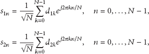
Suppose that each OFDM symbol contains N information symbols. The time-domain OFDM signals transmitted from ${\text{T}}_{\mathrm{1}}$ and ${\text{T}}_{\mathrm{2}}$ after inverse discrete Fourier transform (IDFT) are, respectively, given by

$$\begin{array}{cc}& s_{\mathrm{1}n}=\frac{\mathrm{1}}{\sqrt{N}}\sum _{k=\mathrm{0}}^{N-\mathrm{1}}‍d_{\mathrm{1}k}{e}^{j\mathrm{2}\pi kn/N},\hspace{1em}n=\mathrm{0},\dots ,N-\mathrm{1},\\ s_{\mathrm{2}n}=\frac{\mathrm{1}}{\sqrt{N}}\sum _{k=\mathrm{0}}^{N-\mathrm{1}}‍d_{\mathrm{2}k}{e}^{j\mathrm{2}\pi kn/N},\hspace{1em}n=\mathrm{0},\dots ,N-\mathrm{1},\end{array}$$

(1)

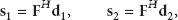
where $\{d_{\mathrm{1}k},\hspace{0.17em}\hspace{0.17em}k=\mathrm{0},\dots ,N-\mathrm{1}\}$ and $\{d_{\mathrm{2}k},k=\mathrm{0},\dots ,N-\mathrm{1}\}$ are zero-mean independent and identically distributed (i.i.d.) data with average power of $P_s$ . Denoting that frequency-domain ${\mathit{d}}_{\mathrm{1}}=[d_{\mathrm{10}},d_{\mathrm{11}},\dots ,d_{\mathrm{1}(N-\mathrm{1})}]$ , ${\mathit{d}}_{\mathrm{2}}=[d_{\mathrm{20}},d_{\mathrm{21}},\dots ,d_{\mathrm{2}(N-\mathrm{1})}]$ and time-domain signals ${\mathit{s}}_{\mathrm{1}}=[s_{\mathrm{10}},s_{\mathrm{11}},\dots ,s_{\mathrm{1}(N-\mathrm{1})}]$ , ${\mathit{s}}_{\mathrm{2}}=[s_{\mathrm{20}},s_{\mathrm{21}},\dots ,s_{\mathrm{2}(N-\mathrm{1})}]$ , the time-domain OFDM signals transmitted from ${\text{T}}_{\mathrm{1}}$ and ${\text{T}}_{\mathrm{2}}$ can be rewritten in vector-matrix form as

$$\begin{array}{cc}& {\mathit{s}}_{\mathrm{1}}={\mathit{F}}^H{\mathit{d}}_{\mathrm{1}},\hspace{1em}\hspace{1em}{\mathit{s}}_{\mathrm{2}}={\mathit{F}}^H{\mathit{d}}_{\mathrm{2}},\end{array}$$

(2)

where F is the normalized DFT matrix whose $(p,q)\text{th}$ entry is $\mathit{F}(i,j)=(\mathrm{1}/\sqrt{N})e^{-j\mathrm{2}\pi ij/N}$ .

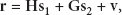
The time-domain symbols $\{s_{\mathrm{1}n},n=\mathrm{0},\dots ,N-\mathrm{1}\}$ and $\{s_{\mathrm{2}n},n=\mathrm{0},\dots ,N-\mathrm{1}\}$ go through regular OFDM transmission steps. Both ${\text{T}}_{\mathrm{1}}$ and ${\text{T}}_{\mathrm{2}}$ insert the cyclic prefix (CP) of length $L_{cp,{\text{T}}_{\mathrm{1}},{\text{T}}_{\mathrm{2}}}\ge \max \{L_h-\mathrm{1},L_g-\mathrm{1}\}$ in front of the OFDM block to avoid intersymbol interference. The time-domain received signal at the relay after removal of CP and DFT is expressed as

$$\begin{array}{l}{r}_n=\frac{\mathrm{1}}{\sqrt{N}}\sum _{k=\mathrm{0}}^{N-\mathrm{1}}‍H_k{d}_{\mathrm{1}k}{e}^{j\mathrm{2}\pi kn/N}+\frac{\mathrm{1}}{\sqrt{N}}\sum _{k=\mathrm{0}}^{N-\mathrm{1}}‍G_k{d}_{\mathrm{2}k}{e}^{j\mathrm{2}\pi kn/N}+v_n,\\ \mathrm{\hspace{0.17em}\hspace{0.17em}}\phantom{=\frac{\mathrm{1}}{\sqrt{N}}\sum _{k=\mathrm{0}}^{N-\mathrm{1}}‍H_k{d}_k{e}^{\frac{j\mathrm{2}\pi kn}{N}}+\frac{\mathrm{1}}{\sqrt{N}}\sum _{k=\mathrm{0}}^{N-\mathrm{1}}‍G_k}n=\mathrm{0},\dots ,N-\mathrm{1},\end{array}$$

(3)

where $H_k$ is the complex gain of the $k\text{th}$ subcarrier of channel h , $G_k$ is the complex gain of the $k\text{th}$ subcarrier of channel g , and $v_n$ is zero-mean circular complex Gaussian with the variance ${\sigma }_v^{\mathrm{2}}$ at the relay. The time-domain received signal at the relay can be rewritten in vector-matrix form as

$$\begin{array}{cc}& \mathit{r}=\mathit{H}{\mathit{s}}_{\mathrm{1}}+\mathit{G}{\mathit{s}}_{\mathrm{2}}+\mathit{v},\end{array}$$

(4)

where $\mathit{r}=[r_{\mathrm{0}},r_{\mathrm{1}},\dots ,r_{(N-\mathrm{1})}]$ , $\mathit{v}=[v_{\mathrm{0}},v_{\mathrm{1}},\dots ,v_{(N-\mathrm{1})}]$ , H is the $N\times N$ circulant matrix whose first column is $[{\mathit{h}}^T,{\mathbf{0}}_{\mathrm{1}\times (N-L_h)}{]}^T$ , and G is the $N\times N$ circulant matrix whose first column is $[{\mathit{g}}^T,{\mathbf{0}}_{\mathrm{1}\times (N-L_g)}{]}^T$ . Define ${\mathrm{\Psi }}_m(\mathit{x})$ as the $N\times m$ column-wise circulant matrix with the first column x ; then we have $\mathit{H}{\mathit{s}}_{\mathrm{1}}={\mathrm{\Psi }}_{L_h}({\mathit{s}}_{\mathrm{1}})\mathit{h}$ and $\mathit{G}{\mathit{s}}_{\mathrm{2}}={\mathrm{\Psi }}_{L_g}({\mathit{s}}_{\mathrm{2}})\mathit{g}$ .

After DFT, the received signal at the relay of the $k\text{th}$ subcarrier is written as

$$\begin{array}{cc}& R_k=H_k{d}_{\mathrm{1}k}+G_k{d}_{\mathrm{2}k}+V_k,\hspace{1em}k=\mathrm{0},\dots ,N-\mathrm{1},\end{array}$$

(5)

where $V_k$ is the corresponding frequency response of the relay noise over the $k\text{th}$ subcarrier with the variance ${\sigma }_V^{\mathrm{2}}$ .

The relay amplifies the received signal $r_n$ , adds a new CP, and forwards the signal ${\mathit{r}}_t=\alpha \mathit{r}$ to ${\text{T}}_{\mathrm{1}}$ and ${\text{T}}_{\mathrm{2}}$ . The relay amplification factor α is chosen as $\sqrt{P_r/({\sigma }_h^{\mathrm{2}}{P}_s+{\sigma }_g^{\mathrm{2}}{P}_s+{\sigma }_n^{\mathrm{2}})}$ . For symmetry, only the process at ${\text{T}}_{\mathrm{1}}$ is discussed. The time-domain received signal at ${\text{T}}_{\mathrm{1}}$ , after CP removal, is

$$\begin{array}{l}{y}_n=\frac{\alpha }{\sqrt{N}}\sum _{k=\mathrm{0}}^{N-\mathrm{1}}‍H_k^{\mathrm{2}}{d}_{\mathrm{1}k}{e}^{j\mathrm{2}\pi kn/N}+\frac{\alpha }{\sqrt{N}}\sum _{k=\mathrm{0}}^{N-\mathrm{1}}‍H_k{G}_k{d}_{\mathrm{2}k}{e}^{j\mathrm{2}\pi kn/N}\\ \hspace{1em}+\frac{\alpha }{\sqrt{N}}\sum _{k=\mathrm{0}}^{N-\mathrm{1}}‍H_k{V}_k{e}^{j\mathrm{2}\pi kn/N}+n_n,\hspace{1em}n=\mathrm{0},\dots ,N-\mathrm{1},\end{array}$$

(6)

where ${\mathit{h}}_{\mathrm{2}}=\mathit{h}\otimes \mathit{g}$ is zero-mean circular complex Gaussian with variance ${\sigma }^{\mathrm{2}}$ at the receiver of ${\text{T}}_{\mathrm{1}}$ . Defining the time-domain cascaded channels ${\mathit{h}}_{\mathrm{1}}=\mathit{h}\otimes \mathit{h}$ and ${\mathit{h}}_{\mathrm{2}}=\mathit{h}\otimes \mathit{g}$ , $\mathit{y}=[y_{\mathrm{0}},y_{\mathrm{1}},\dots ,y_{(N-\mathrm{1})}]$ , $\mathit{n}=[n_{\mathrm{0}},n_{\mathrm{1}},\dots ,n_{(N-\mathrm{1})}]$ , the time-domain received signal at ${\text{T}}_{\mathrm{1}}$ can be rewritten in vector-matrix form as

$$\begin{array}{l}\mathit{y}=\alpha \mathit{H}\mathit{H}{\mathit{s}}_{\mathrm{1}}+\alpha \mathit{H}\mathit{G}{\mathit{s}}_{\mathrm{2}}+\alpha \mathit{H}\mathit{v}+\mathit{n}\\ \hspace{0.17em}\hspace{0.17em}=\alpha {\mathrm{\Psi }}_{\mathrm{2}{L}_h-\mathrm{1}}\left({\mathit{s}}_{\mathrm{1}}\right){\mathit{h}}_{\mathrm{1}}+\alpha {\mathrm{\Psi }}_{L_h+L_g-\mathrm{1}}\left({\mathit{s}}_{\mathrm{2}}\right){\mathit{h}}_{\mathrm{2}}+{\mathit{n}}_a,\end{array}$$

(7)

where ${\mathit{n}}_a=\alpha \mathit{H}\mathit{v}+\mathit{n}$ is the total noise of the receiver at ${\text{T}}_{\mathrm{1}}$ .

After DFT, the received signal at ${\text{T}}_{\mathrm{1}}$ of the $k\text{th}$ subcarrier is written as

$$\begin{array}{l}{Y}_k=\alpha H_k^{\mathrm{2}}{d}_{\mathrm{1}k}+\alpha H_k{G}_k{d}_{\mathrm{2}k}+\alpha H_k{V}_k+N_k,\\ \hspace{1em}\phantom{\text{iiiiiiiiiiiiiiiiiiiiiiiiiiiiiiiiiii}}k=\mathrm{0},\dots ,N-\mathrm{1},\end{array}$$

(8)

where $N_k$ is the corresponding frequency response of the relay noise over the $k\text{th}$ subcarrier. The frequency-domain received signal at ${\text{T}}_{\mathrm{1}}$ can be rewritten in vector-matrix form as

$$\begin{array}{l}\mathit{Y}=\alpha \mathrm{diag}\left\{{\mathit{d}}_{\mathrm{1}}\right\}{\mathit{H}}_{\mathrm{1}}+\alpha \mathrm{diag}\left\{{\mathit{d}}_{\mathrm{2}}\right\}{\mathit{H}}_{\mathrm{2}}+{\mathit{N}}_a\\ \hspace{0.17em}\hspace{0.17em}\hspace{0.17em}=\alpha {\mathit{D}}_{\mathrm{1}}{\mathit{F}}_{\mathrm{2}{L}_h-\mathrm{1}}{\mathit{h}}_{\mathrm{1}}+\alpha {\mathit{D}}_{\mathrm{2}}{\mathit{F}}_{L_h+L_g-\mathrm{1}}{\mathit{h}}_{\mathrm{2}}+{\mathit{N}}_a,\end{array}$$

(9)

where Y is the corresponding frequency response of the time-domain received signal y , ${\mathit{D}}_{\mathrm{1}}=\mathrm{diag}\{{\mathit{d}}_{\mathrm{1}}\}$ , ${\mathit{D}}_{\mathrm{2}}=\mathrm{diag}\{{\mathit{d}}_{\mathrm{2}}\}$ , ${\mathit{N}}_a=\mathit{F}{\mathit{n}}_a$ is the corresponding frequency response of the noise ${\mathit{n}}_a$ , and ${\mathit{N}}_a(k)=\alpha H_k{V}_k+N_k$ . ${\mathit{H}}_{\mathrm{1}}={\mathit{F}}_{\mathrm{2}{L}_h-\mathrm{1}}{\mathit{h}}_{\mathrm{1}}$ and ${\mathit{H}}_{\mathrm{2}}={\mathit{F}}_{L_h+L_g-\mathrm{1}}{\mathit{h}}_{\mathrm{2}}$ are the corresponding frequency responses of the time-domain cascaded channels ${\mathit{h}}_{\mathrm{1}}$ and ${\mathit{h}}_{\mathrm{2}}$ , ${\mathit{H}}_{\mathrm{1}}(k)=H_k^{\mathrm{2}}$ , and ${\mathit{H}}_{\mathrm{2}}(k)=H_k{G}_k$ . ${\mathit{F}}_{\mathrm{2}{L}_h-\mathrm{1}}$ is the first $(\mathrm{2}{L}_h-\mathrm{1})$ column of the DFT matrix F , and ${\mathit{F}}_{L_h+L_g-\mathrm{1}}$ is the first $(L_h+L_g-\mathrm{1})$ column of F . The task of cascaded channel estimation is to find ${\mathit{h}}_{\mathrm{1}}$ and ${\mathit{h}}_{\mathrm{2}}$ from Y .

3. The EM Algorithm Based Channel Estimation

The EM algorithm is a technique for finding maximum likelihood estimates of system parameters in a broad range of problems where observed data are incomplete [19]. The expectation step is performed with respect to unknown underlying parameters, using the current estimate of the parameters, conditioned upon the incomplete observations. The maximization step then provides a new estimate of the parameters that maximizes the expectation of log likelihood function defined over complete data, conditioned on the most recent observation and the last estimate. The EM algorithm consists of two iterative steps: the expectation step and the maximization step. These two steps are iterated until the estimated values converge [20]. When the underlying complete data come from an exponential family whose maximum-likelihood estimates are easily computed, then each maximization step of an EM algorithm is likewise easily computed.

The received signal at the source node in the relay-based M2M two-way communications is a superimposed signal, which can be decomposed into two signal components with two unknown channel parameters, one is the self-interference signal, and the other is the desired signal from the other source node. Take the channel estimation at source node 1, for example, the two unknown parameters are source1-relay-source1 cascaded channel and source2-relay-source1 cascaded channel. The source1-relay-source1 channel is the unobserved data when estimating source2-relay-source1 channel, while the source2-relay-source1 channel is also the unobserved data when estimating source1-relay-source1 channel. Since the superimposed signal structure at the receiver is conducive to the application of the EM algorithm and the closed-form solution of maximum likelihood channel estimation does not exist, the EM algorithm is utilized to provide the maximum likelihood solution in the presence of unobserved data through stable iterations.

In the EM channel estimation, the set of unknown parameters is $\theta =\{{\mathit{h}}_{\mathrm{1}},{\mathit{h}}_{\mathrm{2}}\}$ , the received signal Y / y at ${\text{T}}_{\mathrm{1}}$ is treated as the observed (incomplete) data, and the set of the two signal components from the two source nodes is modeled as the complete data. Conditioned upon the incomplete observations, the algorithm maximizes the expectation of log likelihood function defined over the complete data, by averaging over the unknown underlying parameters and using the current estimate of the parameters.

3.1. Cascaded Channel Estimation Based on Frequency Domain Processing

The frequency-domain received signal Y at ${\text{T}}_{\mathrm{1}}$ , also the incomplete data, can be written as

$$\begin{array}{cc}& \mathit{Y}=\alpha {\mathit{D}}_{\mathrm{1}}{\mathit{F}}_{\mathrm{2}{L}_h-\mathrm{1}}{\mathit{h}}_{\mathrm{1}}+\alpha {\mathit{D}}_{\mathrm{2}}{\mathit{F}}_{L_h+L_g-\mathrm{1}}{\mathit{h}}_{\mathrm{2}}+{\mathit{N}}_a.\end{array}$$

(10)

A natural choice for the complete data ${\mathit{Y}}_c$ is obtained by decomposing the observed data Y into its signal components:

$$\begin{array}{cc}& {\mathit{Y}}_c=\left[\begin{array}{c}{\mathit{Y}}_{\mathrm{1}}\\ {\mathit{Y}}_{\mathrm{2}}\end{array}\right]=\left[\begin{array}{c}\alpha {\mathit{D}}_{\mathrm{1}}{\mathit{F}}_{\mathrm{2}{L}_h-\mathrm{1}}{\mathit{h}}_{\mathrm{1}}+{\mathit{N}}_{\mathrm{1}}\\ \alpha {\mathit{D}}_{\mathrm{2}}{\mathit{F}}_{L_h+L_g-\mathrm{1}}{\mathit{h}}_{\mathrm{2}}+{\mathit{N}}_{\mathrm{2}}\end{array}\right],\end{array}$$

(11)

where ${\mathit{Y}}_{\mathrm{1}}$ is the component of the received signal Y transmitted by the source node ${\text{T}}_{\mathrm{1}}$ through the channel with impulse response ${\mathit{h}}_{\mathrm{1}}$ , ${\mathit{Y}}_{\mathrm{2}}$ is the component of the received signal Y transmitted by the source node ${\text{T}}_{\mathrm{2}}$ through the channel with impulse response ${\mathit{h}}_{\mathrm{2}}$ . ${\mathit{N}}_{\mathrm{1}}$ and ${\mathit{N}}_{\mathrm{2}}$ are obtained by arbitrarily decomposing the total noise ${\mathit{N}}_a$ into two components:

$$\begin{array}{cc}& {\mathit{N}}_{\mathrm{1}}+{\mathit{N}}_{\mathrm{2}}={\mathit{N}}_a.\end{array}$$

(12)

It is found to be most convenient to let ${\mathit{N}}_{\mathrm{1}}$ and ${\mathit{N}}_{\mathrm{2}}$ be statistically independent, zero-mean, and Gaussian with the covariance matrix ${\mathit{R}}_{\mathrm{1}}$ and ${\mathit{R}}_{\mathrm{2}}$ , respectively. Denote the covariance matrix of ${\mathit{N}}_a$ as ${\mathit{R}}_a$ ; then ${\mathit{R}}_{\mathrm{1}}+{\mathit{R}}_{\mathrm{2}}={\mathit{R}}_a$ .

The log-likelihood of the complete data ${\mathit{Y}}_c$ is

$$\begin{array}{cc}& \log p\left({\mathit{Y}}_c\hspace{0.17em}|\hspace{0.17em}\theta \right)=c-{\left({\mathit{Y}}_c-{\mathit{D}}_c\right)}^H{\mathrm{\Lambda }}^{-\mathrm{1}}\left({\mathit{Y}}_c-{\mathit{D}}_c\right),\end{array}$$

(13)

where c contains all the terms that are independent of $\theta =\{{\mathit{h}}_{\mathrm{1}},{\mathit{h}}_{\mathrm{2}}\}$ and the mean vector ${\mathit{D}}_c$ and the covariance matrix Λ are given, respectively, by

$$\begin{array}{cc}& {\mathit{D}}_c=\left[\begin{array}{c}\alpha {\mathit{D}}_{\mathrm{1}}{\mathit{F}}_{\mathrm{2}{L}_h-\mathrm{1}}{\mathit{h}}_{\mathrm{1}}\\ \alpha {\mathit{D}}_{\mathrm{2}}{\mathit{F}}_{L_h+L_g-\mathrm{1}}{\mathit{h}}_{\mathrm{2}}\end{array}\right],\\ \mathrm{\Lambda }=\left[\begin{array}{cc}{\mathit{R}}_{\mathrm{1}}& \mathbf{0}\\ \mathbf{0}& {\mathit{R}}_{\mathrm{2}}\end{array}\right]=\left[\begin{array}{cc}{\beta }_{\mathrm{1}}{\mathit{R}}_{\mathit{n}\hspace{0.17em}|\hspace{0.17em}\theta }& \mathit{0}\\ \mathit{0}& {\beta }_{\mathrm{2}}{\mathit{R}}_{\mathit{n}\hspace{0.17em}|\hspace{0.17em}\theta }\end{array}\right],\end{array}$$

(14)

where ${\beta }_{\mathrm{1}}$ and ${\beta }_{\mathrm{2}}$ are both real numbers, $\mathrm{0}<{\beta }_{\mathrm{1}}<\mathrm{1}$ , $\mathrm{0}<{\beta }_{\mathrm{2}}<\mathrm{1}$ , and ${\beta }_{\mathrm{1}}+{\beta }_{\mathrm{2}}=\mathrm{1}$ .

Suppose that ${\widehat{\theta }}^{(i)}=\{{\widehat{\mathit{h}}}_{\mathrm{1}}^{(i)},{\widehat{\mathit{h}}}_{\mathrm{2}}^{(i)}\}$ denotes the current value of $\theta =\{{\mathit{h}}_{\mathrm{1}},{\mathit{h}}_{\mathrm{2}}\}$ after i iterations of the EM algorithm. The $(i+\mathrm{1})\text{th}$ iteration can be described in two steps as follows.

(1) E-step: given the observations Y and the last estimates ${\widehat{\theta }}^{(i)}=\{{\widehat{\mathit{h}}}_{\mathrm{1}}^{(i)},{\widehat{\mathit{h}}}_{\mathrm{2}}^{(i)}\}$ , compute the expectation $Q(\theta \hspace{0.17em}|\hspace{0.17em}{\widehat{\theta }}^{(i)})$ of the log-likelihood of the complete data ${\mathit{Y}}_c$ , which is also the conditional expectation of (13),

$$\begin{array}{l}Q\left(\theta \hspace{0.17em}|\hspace{0.17em}{\widehat{\theta }}^{\left(i\right)}\right)=\text{E}\left[\log p\left({\mathit{Y}}_c\hspace{0.17em}|\hspace{0.17em}\theta \right)\hspace{0.17em}|\hspace{0.17em}\mathit{Y},{\widehat{\theta }}^{\left(i\right)}\right]\\ \hspace{1em}\hspace{1em}\hspace{1em}\hspace{1em}\hspace{0.17em}\hspace{0.17em}=d-{\left({\widehat{\mathit{Y}}}_c^{\left(i\right)}-{\mathit{D}}_c\right)}^H{\mathrm{\Lambda }}^{-\mathrm{1}}\left({\widehat{\mathit{Y}}}_c^{\left(i\right)}-{\mathit{D}}_c\right),\end{array}$$

(15)

where d contains all the terms that are independent of $\theta =\{{\mathit{h}}_{\mathrm{1}},{\mathit{h}}_{\mathrm{2}}\}$ , and the $i\text{th}$ estimate of the conditional expectation of the complete data ${\mathit{Y}}_c$ is [25]

$$\begin{array}{l}{\widehat{\mathit{Y}}}_c^{\left(i\right)}={\text{E}}_{}\left\{{\mathit{Y}}_c\hspace{0.17em}|\hspace{0.17em}\mathit{Y},{\widehat{\theta }}^{\left(i\right)}\right\}\\ \hspace{1em}\hspace{1em}=\left\{\left[\begin{array}{l}{\mathit{Y}}_{\mathrm{1}}\\ {\mathit{Y}}_{\mathrm{2}}\end{array}\right]\hspace{0.17em}|\hspace{0.17em}{\widehat{\theta }}^{\left(i\right)}\right\}+\left[\begin{array}{l}{\beta }_{\mathrm{1}}{\mathit{R}}_{\mathit{n}\hspace{0.17em}|\hspace{0.17em}\theta }\\ {\beta }_{\mathrm{2}}{\mathit{R}}_{\mathit{n}\hspace{0.17em}|\hspace{0.17em}\theta }\end{array}\right]{\mathit{R}}_{\mathit{n}\hspace{0.17em}|\hspace{0.17em}\theta }^{-\mathrm{1}}\\ \hspace{1em}\hspace{1em}\hspace{1em}\times \left[\mathit{Y}-\mathit{A}{\text{E}}_{}\left\{{\mathit{Y}}_c\hspace{0.17em}|\hspace{0.17em}{\widehat{\theta }}^{\left(i\right)}\right\}\right].\end{array}$$

(16)

$Q(\theta \hspace{0.17em}|\hspace{0.17em}{\widehat{\theta }}^{(i)})$ contains both the unknown variable $\theta =\{{\mathit{h}}_{\mathrm{1}},{\mathit{h}}_{\mathrm{2}}\}$ and the known constant ${\widehat{\theta }}^{(i)}=\{{\widehat{\mathit{h}}}_{\mathrm{1}}^{(i)},{\widehat{\mathit{h}}}_{\mathrm{2}}^{(i)}\}$ . The conditional expectations of ${\mathit{Y}}_{\mathrm{1}}$ and ${\mathit{Y}}_{\mathrm{2}}$ are given, respectively, by

$$\begin{array}{l}{\widehat{\mathit{Y}}}_{\mathrm{1}}^{\left(i\right)}=\alpha {\mathit{D}}_{\mathrm{1}}{\mathit{F}}_{\mathrm{2}{L}_h-\mathrm{1}}{\widehat{\mathit{h}}}_{\mathrm{1}}^{\left(i\right)}+{\beta }_{\mathrm{1}}\\ \hspace{1em}\hspace{0.17em}\hspace{1em}\times \left[\mathit{Y}-\alpha {\mathit{D}}_{\mathrm{1}}{\mathit{F}}_{\mathrm{2}{L}_h-\mathrm{1}}{\widehat{\mathit{h}}}_{\mathrm{1}}^{\left(i\right)}-\alpha {\mathit{D}}_{\mathrm{2}}{\mathit{F}}_{L_h+L_g-\mathrm{1}}{\widehat{\mathit{h}}}_{\mathrm{2}}^{\left(i\right)}\right],\\ {\widehat{\mathit{Y}}}_{\mathrm{2}}^{\left(i\right)}=\alpha {\mathit{D}}_{\mathrm{2}}{\mathit{F}}_{L_h+L_g-\mathrm{1}}{\widehat{\mathit{h}}}_{\mathrm{2}}^{\left(i\right)}+{\beta }_{\mathrm{2}}\\ \hspace{1em}\hspace{0.17em}\hspace{1em}\times \left[\mathit{Y}-\alpha {\mathit{D}}_{\mathrm{1}}{\mathit{F}}_{\mathrm{2}{L}_h-\mathrm{1}}{\widehat{\mathit{h}}}_{\mathrm{1}}^{\left(i\right)}-\alpha {\mathit{D}}_{\mathrm{2}}{\mathit{F}}_{L_h+L_g-\mathrm{1}}{\widehat{\mathit{h}}}_{\mathrm{2}}^{\left(i\right)}\right].\end{array}$$

(17)

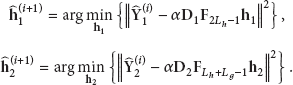
(2) M-step: maximize the conditional expectation $Q(\theta \hspace{0.17em}|\hspace{0.17em}{\widehat{\theta }}^{(i)})$ of the log-likelihood of the complete data ${\mathit{Y}}_c$ ,

$$\begin{array}{l}{\widehat{\theta }}^{\left(i+\mathrm{1}\right)}=\arg \underset{\theta }{\max }Q\left(\theta \hspace{0.17em}|\hspace{0.17em}{\widehat{\theta }}^{\left(i\right)}\right)\\ \hspace{1em}\hspace{1em}=\arg \underset{\theta }{\max }\left[-{\left({\widehat{\mathit{Y}}}_c^{\left(i\right)}-{\mathit{D}}_c\right)}^H{\mathrm{\Lambda }}^{-\mathrm{1}}\left({\widehat{\mathit{Y}}}_c^{\left(i\right)}-{\mathit{D}}_c\right)\right],\end{array}$$

(18)

which is equivalent to solve

$$\begin{array}{cc}& {\widehat{\mathit{h}}}_{\mathrm{1}}^{\left(i+\mathrm{1}\right)}=\arg \underset{{\mathit{h}}_{\mathrm{1}}}{\min }\left\{{\parallel {\widehat{\mathit{Y}}}_{\mathrm{1}}^{\left(i\right)}-\alpha {\mathit{D}}_{\mathrm{1}}{\mathit{F}}_{\mathrm{2}{L}_h-\mathrm{1}}{\mathit{h}}_{\mathrm{1}}\parallel }^2\right\},\\ {\widehat{\mathit{h}}}_{\mathrm{2}}^{\left(i+\mathrm{1}\right)}=\arg \underset{{\mathit{h}}_{\mathrm{2}}}{\min }\left\{{\parallel {\widehat{\mathit{Y}}}_{\mathrm{2}}^{\left(i\right)}-\alpha {\mathit{D}}_{\mathrm{2}}{\mathit{F}}_{L_h+L_g-\mathrm{1}}{\mathit{h}}_{\mathrm{2}}\parallel }^2\right\}.\end{array}$$

(19)

We obtain

$$\begin{array}{cc}& {\widehat{\mathit{h}}}_{\mathrm{1}}^{\left(i+\mathrm{1}\right)}=\frac{\mathrm{1}}{\alpha }{\mathit{F}}_{\mathrm{2}{L}_h-\mathrm{1}}^H{\mathit{D}}_{\mathrm{1}}^{-\mathrm{1}}{\widehat{\mathit{Y}}}_{\mathrm{1}}^{\left(i\right)},\\ {\widehat{\mathit{h}}}_{\mathrm{2}}^{\left(i+\mathrm{1}\right)}=\frac{\mathrm{1}}{\alpha }{\mathit{F}}_{L_h+L_g-\mathrm{1}}^H{\mathit{D}}_{\mathrm{2}}^{-\mathrm{1}}{\widehat{\mathit{Y}}}_{\mathrm{2}}^{\left(i\right)}.\end{array}$$

(20)

The new estimates ${\widehat{\theta }}^{(i+\mathrm{1})}=\{{\widehat{\mathit{h}}}_{\mathrm{1}}^{(i+\mathrm{1})},{\widehat{\mathit{h}}}_{\mathrm{2}}^{(i+\mathrm{1})}\}$ are utilized in the E-step of the next iteration to update ${\widehat{\mathit{Y}}}_{\mathrm{1}}^{(i+\mathrm{1})}$ and ${\widehat{\mathit{Y}}}_{\mathrm{2}}^{(i+\mathrm{1})}$ . Each iteration cycle increases the likelihood until convergence is accomplished.

The most striking feature of the algorithm is that it decouples the multiple-input channel estimation problem into two separate single-input channel estimation problems, a much more palatable problem. Therefore, the complexity of the channel estimation algorithm is essentially unaffected by the assumed number of signal components. Since F and ${\mathit{F}}^H$ are DFT matrices and ${\mathit{D}}_{\mathrm{1}}$ and ${\mathit{D}}_{\mathrm{2}}$ are diagonal matrices, the matrix inversion operation is relatively simple.

3.2. Cascaded Channel Estimation Based on Time Domain Processing

The time-domain received signal y at ${\text{T}}_{\mathrm{1}}$ can be written as

$$\begin{array}{cc}& \mathit{y}=\alpha {\mathrm{\Psi }}_{\mathrm{2}{L}_h-\mathrm{1}}\left({\mathit{s}}_{\mathrm{1}}\right){\mathit{h}}_{\mathrm{1}}+\alpha {\mathrm{\Psi }}_{L_h+L_g-\mathrm{1}}\left({\mathit{s}}_{\mathrm{2}}\right){\mathit{h}}_{\mathrm{2}}+{\mathit{n}}_a.\end{array}$$

(21)

A natural choice for the complete data ${\mathit{y}}_c$ is obtained by decomposing the observed data y into its signal components:

$$\begin{array}{cc}& {\mathit{y}}_c=\left[\begin{array}{c}{\mathit{y}}_{\mathrm{1}}\\ {\mathit{y}}_{\mathrm{2}}\end{array}\right]=\left[\begin{array}{c}\alpha {\mathrm{\Psi }}_{\mathrm{2}{L}_h-\mathrm{1}}\left({\mathit{s}}_{\mathrm{1}}\right){\mathit{h}}_{\mathrm{1}}+{\mathit{n}}_{\mathrm{1}}\\ \alpha {\mathrm{\Psi }}_{L_h+L_g-\mathrm{1}}\left({\mathit{s}}_{\mathrm{2}}\right){\mathit{h}}_{\mathrm{2}}+{\mathit{n}}_{\mathrm{2}}\end{array}\right],\end{array}$$

(22)

where ${\mathit{y}}_{\mathrm{1}}$ is the component of the received signal y transmitted by the source node ${\text{T}}_{\mathrm{1}}$ through the channel with impulse response ${\mathit{h}}_{\mathrm{1}}$ , ${\mathit{y}}_{\mathrm{2}}$ is the component of the received signal y transmitted by the source node ${\text{T}}_{\mathrm{2}}$ through the channel with impulse response ${\mathit{h}}_{\mathrm{2}}$ , and ${\mathit{n}}_{\mathrm{1}}$ and ${\mathit{n}}_{\mathrm{2}}$ are obtained by arbitrarily decomposing the total noise ${\mathit{n}}_a$ into two components:

$$\begin{array}{cc}& {\mathit{n}}_{\mathrm{1}}+{\mathit{n}}_{\mathrm{2}}={\mathit{n}}_a.\end{array}$$

(23)

Let ${\mathit{n}}_{\mathrm{1}}$ and ${\mathit{n}}_{\mathrm{2}}$ be statistically independent, zero-mean, and Gaussian with the covariance matrix ${\mathit{R}}_{\mathrm{1}}$ and ${\mathit{R}}_{\mathrm{2}}$ , respectively. Denote the covariance matrix of ${\mathit{n}}_a$ as ${\mathit{R}}_a$ ; then ${\mathit{R}}_{\mathrm{1}}+{\mathit{R}}_{\mathrm{2}}={\mathit{R}}_a$ .

The log-likelihood of the complete data ${\mathit{y}}_c$ is

$$\begin{array}{cc}& \log p\left({\mathit{y}}_c\hspace{0.17em}|\hspace{0.17em}\theta \right)=c-{\left({\mathit{y}}_c-{\mathit{s}}_c\right)}^H{\mathrm{\Lambda }}^{-\mathrm{1}}\left({\mathit{y}}_c-{\mathit{s}}_c\right),\end{array}$$

(24)

where c contains all the terms that are independent of $\theta =\{{\mathit{h}}_{\mathrm{1}},{\mathit{h}}_{\mathrm{2}}\}$ and the mean vector ${\mathit{s}}_c$ and the covariance matrix Λ are given, respectively, by

$$\begin{array}{cc}& {\mathit{s}}_c=\left[\begin{array}{c}\alpha {\mathrm{\Psi }}_{\mathrm{2}{L}_h-\mathrm{1}}\left({\mathit{s}}_{\mathrm{1}}\right){\mathit{h}}_{\mathrm{1}}\\ \alpha {\mathrm{\Psi }}_{L_h+L_g-\mathrm{1}}\left({\mathit{s}}_{\mathrm{2}}\right){\mathit{h}}_{\mathrm{2}}\end{array}\right],\\ \mathrm{\Lambda }=\left[\begin{array}{cc}{\mathit{R}}_{\mathrm{1}}& \mathit{0}\\ \mathit{0}& {\mathit{R}}_{\mathrm{2}}\end{array}\right]=\left[\begin{array}{cc}{\beta }_{\mathrm{1}}{\mathit{R}}_{\mathit{n}\hspace{0.17em}|\hspace{0.17em}\theta }& \mathit{0}\\ \mathit{0}& {\beta }_{\mathrm{2}}{\mathit{R}}_{\mathit{n}\hspace{0.17em}|\hspace{0.17em}\theta }\end{array}\right],\end{array}$$

(25)

where ${\beta }_{\mathrm{1}}$ and ${\beta }_{\mathrm{2}}$ are both real numbers, $\mathrm{0}<{\beta }_{\mathrm{1}}<\mathrm{1}$ , $\mathrm{0}<{\beta }_{\mathrm{2}}<\mathrm{1}$ , ${\beta }_{\mathrm{1}}+{\beta }_{\mathrm{2}}=\mathrm{1}$ .

Suppose that ${\widehat{\theta }}^{(i)}=\{{\widehat{\mathit{h}}}_{\mathrm{1}}^{(i)},{\widehat{\mathit{h}}}_{\mathrm{2}}^{(i)}\}$ denotes the current value of $\theta =\{{\mathit{h}}_{\mathrm{1}},{\mathit{h}}_{\mathrm{2}}\}$ after i iterations of the EM algorithm. The $(i+\mathrm{1})\text{th}$ iteration can be described in two steps as follows.

(1) E-step: given the observations y and the last estimates ${\widehat{\theta }}^{(i)}=\{{\widehat{\mathit{h}}}_{\mathrm{1}}^{(i)},{\widehat{\mathit{h}}}_{\mathrm{2}}^{(i)}\}$ , compute the expectation $Q(\theta \hspace{0.17em}|\hspace{0.17em}{\widehat{\theta }}^{(i)})$ of the log-likelihood of the complete data ${\mathit{y}}_c$ , which is also the conditional expectation of (24),

$$\begin{array}{cc}& Q(\theta \hspace{0.17em}|\hspace{0.17em}{\widehat{\theta }}^{\left(i\right)}=d-{\left({\widehat{\mathit{y}}}_c^{\left(i\right)}-{\mathit{s}}_c\right)}^H{\mathrm{\Lambda }}^{-\mathrm{1}}\left({\widehat{\mathit{y}}}_c^{\left(i\right)}-{\mathit{s}}_c\right),\end{array}$$

(26)

where d contains all the terms that are independent of $\theta =\{{\mathit{h}}_{\mathrm{1}},{\mathit{h}}_{\mathrm{2}}\}$ and the $i\text{th}$ estimate of the conditional expectation of the complete data ${\mathit{y}}_c$ is [23]

$$\begin{array}{l}{\widehat{\mathit{y}}}_c^{\left(i\right)}=\text{E}\left\{\left[\begin{array}{l}{\mathit{y}}_{\mathrm{1}}\\ {\mathit{y}}_{\mathrm{2}}\end{array}\right]\hspace{0.17em}|\hspace{0.17em}{\widehat{\theta }}^{\left(i\right)}\right\}+\left[\begin{array}{l}{\beta }_{\mathrm{1}}{\mathit{R}}_{\mathit{n}\hspace{0.17em}|\hspace{0.17em}\theta }\\ {\beta }_{\mathrm{2}}{\mathit{R}}_{\mathit{n}\hspace{0.17em}|\hspace{0.17em}\theta }\end{array}\right]{\mathit{R}}_{\mathit{n}\hspace{0.17em}|\hspace{0.17em}\theta }^{-\mathrm{1}}\\ \hspace{1em}\hspace{1em}\times \left[\mathit{y}-\mathit{A}\text{E}\left\{{\mathit{y}}_c\hspace{0.17em}|\hspace{0.17em}{\widehat{\theta }}^{\left(i\right)}\right\}\right].\end{array}$$

(27)

The conditional expectations of ${\mathbf{y}}_{\mathrm{1}}$ and ${\mathbf{y}}_{\mathrm{2}}$ are given, respectively, by

$$\begin{array}{l}{\widehat{\mathit{y}}}_{\mathrm{1}}^{\left(i\right)}=\alpha {\mathrm{\Psi }}_{\mathrm{2}{L}_h-\mathrm{1}}\left({\mathit{s}}_{\mathrm{1}}\right){\widehat{\mathit{h}}}_{\mathrm{1}}^{\left(i\right)}+{\beta }_{\mathrm{1}}\\ \hspace{1em}\hspace{1em}\times \left[\mathit{y}-\alpha {\mathrm{\Psi }}_{\mathrm{2}{L}_h-\mathrm{1}}\left({\mathit{s}}_{\mathrm{1}}\right){\widehat{\mathit{h}}}_{\mathrm{1}}^{\left(i\right)}-\alpha {\mathrm{\Psi }}_{L_h+L_g-\mathrm{1}}\left({\mathit{s}}_{\mathrm{2}}\right){\widehat{\mathit{h}}}_{\mathrm{2}}^{\left(i\right)}\right],\\ {\widehat{\mathit{y}}}_{\mathrm{2}}^{\left(i\right)}=\alpha {\mathrm{\Psi }}_{L_h+L_g-\mathrm{1}}\left({\mathit{s}}_{\mathrm{2}}\right){\widehat{\mathit{h}}}_{\mathrm{2}}^{\left(i\right)}+{\beta }_{\mathrm{2}}\\ \hspace{1em}\hspace{1em}\times \left[\mathit{y}-\alpha {\mathrm{\Psi }}_{\mathrm{2}{L}_h-\mathrm{1}}\left({\mathit{s}}_{\mathrm{1}}\right){\widehat{\mathit{h}}}_{\mathrm{1}}^{\left(i\right)}-\alpha {\mathrm{\Psi }}_{L_h+L_g-\mathrm{1}}\left({\mathit{s}}_{\mathrm{2}}\right){\widehat{\mathit{h}}}_{\mathrm{2}}^{\left(i\right)}\right].\end{array}$$

(28)

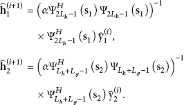
(2) M-step: maximize the conditional expectation $Q(\theta \hspace{0.17em}|\hspace{0.17em}{\widehat{\theta }}^{(i)})$ ,

$$\begin{array}{cc}& {\widehat{\theta }}^{\left(i+\mathrm{1}\right)}=\arg \underset{\theta }{\max }\left[-{\left({\widehat{\mathit{y}}}_c^{\left(i\right)}-{\mathit{s}}_c\right)}^H{\mathrm{\Lambda }}^{-\mathrm{1}}\left({\widehat{\mathit{y}}}_c^{\left(i\right)}-{\mathit{s}}_c\right)\right].\end{array}$$

(29)

We obtain

$$\begin{array}{l}{\widehat{\mathit{h}}}_{\mathrm{1}}^{\left(i+\mathrm{1}\right)}={\left(\alpha {\mathrm{\Psi }}_{\mathrm{2}{L}_h-\mathrm{1}}^H\left({\mathit{s}}_{\mathrm{1}}\right){\mathrm{\Psi }}_{\mathrm{2}{L}_h-\mathrm{1}}\left({\mathit{s}}_{\mathrm{1}}\right)\right)}^{-\mathrm{1}}\\ \hspace{1em}\hspace{1em}\hspace{1em}\times {\mathrm{\Psi }}_{\mathrm{2}{L}_h-\mathrm{1}}^H\left({\mathit{s}}_{\mathrm{1}}\right){\widehat{\mathit{y}}}_{\mathrm{1}}^{\left(i\right)},\\ {\widehat{\mathit{h}}}_{\mathrm{2}}^{\left(i+\mathrm{1}\right)}={\left(\alpha {\mathrm{\Psi }}_{L_h+L_g-\mathrm{1}}^H\left({\mathit{s}}_{\mathrm{2}}\right){\mathrm{\Psi }}_{L_h+L_g-\mathrm{1}}\left({\mathit{s}}_{\mathrm{2}}\right)\right)}^{-\mathrm{1}}\\ \hspace{1em}\hspace{1em}\hspace{1em}\times {\mathrm{\Psi }}_{L_h+L_g-\mathrm{1}}^H\left({\mathit{s}}_{\mathrm{2}}\right){\widehat{\mathit{y}}}_{\mathrm{2}}^{\left(i\right)}.\end{array}$$

(30)

The new estimates ${\widehat{\theta }}^{(i+\mathrm{1})}=\{{\widehat{\mathit{h}}}_{\mathrm{1}}^{(i+\mathrm{1})},{\widehat{\mathit{h}}}_{\mathrm{2}}^{(i+\mathrm{1})}\}$ are utilized in the E-step of the next iteration to update ${\widehat{\mathit{y}}}_{\mathrm{1}}^{(i+\mathrm{1})}$ and ${\widehat{\mathit{y}}}_{\mathrm{2}}^{(i+\mathrm{1})}$ . Each iteration cycle increases the likelihood until convergence is accomplished.

3.3. Cascaded Channel Estimation without Training Sequence

In Sections 3.1 and 3.2, the channel estimate is continuously updated by transmitting pilot symbols using specified time-frequency lattices. When no training sequence is available and signals are still to be detected from the observations, the EM algorithm is applied to take an average over the unknown channel impulse response for reducing bit errors caused by uncertainty in the channel. Here no training sequence means that the source node ${\text{T}}_{\mathrm{1}}$ only knows its own signals ${\mathit{d}}_{\mathrm{1}}$ , while ${\mathit{d}}_{\mathrm{2}}$ is completely unknown to ${\text{T}}_{\mathrm{1}}$ .

The selection of the complete data ${\mathit{Y}}_c$ is the same as Section 3.1, and the log-likelihood of the complete data ${\mathit{Y}}_c$ is the same as (13).

Suppose that ${\widehat{\theta }}^{(i)}=\{{\widehat{\mathit{h}}}_{\mathrm{1}}^{(i)},{\widehat{\mathit{h}}}_{\mathrm{2}}^{(i)}\}$ denotes the current value of $\theta =\{{\mathit{h}}_{\mathrm{1}},{\mathit{h}}_{\mathrm{2}}\}$ after i iterations of the EM algorithm. The $(i+\mathrm{1})\text{th}$ iteration can be described in two steps as follows.

(1) E-step: given the observations Y and the last estimates ${\widehat{\theta }}^{(i)}=\{{\widehat{\mathit{h}}}_{\mathrm{1}}^{(i)},{\widehat{\mathit{h}}}_{\mathrm{2}}^{(i)}\}$ , compute the expectation $Q(\theta \hspace{0.17em}|\hspace{0.17em}{\widehat{\theta }}^{(i)})$ of the log-likelihood of the complete data ${\mathit{Y}}_c$ , which is the conditional expectation of (13)

$$\begin{array}{cc}& Q\left(\theta \hspace{0.17em}|\hspace{0.17em}{\widehat{\theta }}^{\left(i\right)}\right)=d-{\left({\widehat{\mathit{Y}}}_c^{\left(i\right)}-{\mathit{D}}_c\right)}^H{\mathrm{\Lambda }}^{-\mathrm{1}}\left({\widehat{\mathit{Y}}}_c^{\left(i\right)}-{\mathit{D}}_c\right),\end{array}$$

(31)

where d contains all the terms that are independent of $\theta =\{{\mathit{h}}_{\mathrm{1}},{\mathit{h}}_{\mathrm{2}}\}$ and the $i\text{th}$ estimate of the conditional expectations of ${\mathit{Y}}_{\mathrm{1}}$ and ${\mathit{Y}}_{\mathrm{2}}$ are given, respectively, by [23]

$$\begin{array}{l}{\widehat{\mathit{Y}}}_{\mathrm{1}}^{\left(i\right)}=\alpha {\mathit{D}}_{\mathrm{1}}{\mathit{F}}_{\mathrm{2}{L}_h-\mathrm{1}}{\widehat{\mathit{h}}}_{\mathrm{1}}^{\left(i\right)}+{\beta }_{\mathrm{1}}\\ \hspace{1em}\hspace{1em}\hspace{1em}\times \left[\mathit{Y}-\alpha {\mathit{D}}_{\mathrm{1}}{\mathit{F}}_{\mathrm{2}{L}_h-\mathrm{1}}{\widehat{\mathit{h}}}_{\mathrm{1}}^{\left(i\right)}-\alpha {\widehat{\mathit{D}}}_{\mathrm{2}}^{\left(i\right)}{\mathit{F}}_{L_h+L_g-\mathrm{1}}{\widehat{\mathit{h}}}_{\mathrm{2}}^{\left(i\right)}\right],\\ {\widehat{\mathit{Y}}}_{\mathrm{2}}^{\left(i\right)}=\alpha {\widehat{\mathit{D}}}_{\mathrm{2}}^{\left(i\right)}{\mathit{F}}_{L_h+L_g-\mathrm{1}}{\widehat{\mathit{h}}}_{\mathrm{2}}^{\left(i\right)}+{\beta }_{\mathrm{2}}\\ \hspace{1em}\hspace{1em}\hspace{1em}\times \left[\mathit{Y}-\alpha {\mathit{D}}_{\mathrm{1}}{\mathit{F}}_{\mathrm{2}{L}_h-\mathrm{1}}{\widehat{\mathit{h}}}_{\mathrm{1}}^{\left(i\right)}-\alpha {\widehat{\mathit{D}}}_{\mathrm{2}}^{\left(i\right)}{\mathit{F}}_{L_h+L_g-\mathrm{1}}{\widehat{\mathit{h}}}_{\mathrm{2}}^{\left(i\right)}\right],\end{array}$$

(32)

where ${\widehat{\mathit{D}}}_{\mathrm{2}}^{(i)}$ is the estimate of ${\mathit{D}}_{\mathrm{2}}$ in the $i\text{th}$ iteration,

$$\begin{array}{l}\hspace{1em}\hspace{1em}\hspace{1em}{\widehat{\mathit{D}}}_{\mathrm{2}}^{\left(i\right)}=\text{E}\left\{{\mathit{D}}_{\mathrm{2}}\hspace{0.17em}|\hspace{0.17em}\mathit{y},{\widehat{\theta }}^{\left(i\right)}\right\}=\mathrm{diag}\left\{{\widehat{\mathit{d}}}_{\mathrm{2}}^{\left(i\right)}\right\},\\ \hspace{1em}\hspace{1em}{\widehat{\mathit{d}}}_{\mathrm{2}}^{\left(i\right)}={\left[{\widehat{d}}_{\mathrm{2}}^{\left(i\right)}\left(\mathrm{0}\right),{\widehat{d}}_{\mathrm{2}}^{\left(i\right)}\left(\mathrm{1}\right),\dots ,{\widehat{d}}_{\mathrm{2}}^{\left(i\right)}\left(N-\mathrm{1}\right)\right]}^T,\\ {\widehat{d}}_{\mathrm{2}}^{\left(i\right)}\left(n\right)=\sum _{m=\mathrm{1}}^M‍{\rho }_m^{\left(i\right)}\left(n\right)s_m,\hspace{1em}\hspace{1em}{\widehat{d}}_{\mathrm{2}m}^{\left(i\right)}\left(n\right)=s_m,\hspace{1em}\hspace{1em}{\widehat{d}}_{\mathrm{2}j}^{\left(i\right)}\left(n\right)=s_j,\\ {\rho }_m^{\left(i\right)}\left(n\right)=\left(\exp \left\{-{\left(Y\left(n\right)-{\mu }^{\left(i\right)}\left(n\right)\right)}^H{\mathit{R}}_{\mathit{n}|\theta }^{-\mathrm{1}}\left(Y\left(n\right)-{\mu }^{\left(i\right)}\left(n\right)\right)\right\}\right)\\ \hspace{1em}\hspace{1em}\times ({\sum }_{j=\mathrm{1}}^M‍\exp \{-{\left(Y\left(n\right)-{\mu }_j^{\left(i\right)}\left(n\right)\right)}^H\\ \hspace{1em}\hspace{1em}\hspace{1em}\hspace{1em}\hspace{1em}\hspace{1em}\times {{\mathit{R}}_{\mathit{n}|\theta }^{-\mathrm{1}}\left(Y\left(n\right)-{\mu }_j^{\left(i\right)}\left(n\right)\right)\phantom{{\left(Y\left(n\right)-{\mu }_j^{\left(i\right)}\left(n\right)\right)}^H}\}\phantom{{\sum }_{j=\mathrm{1}}^M‍})}^{-1},\\ \hspace{1em}\hspace{1em}\hspace{1em}\hspace{1em}{\mu }^{\left(i\right)}\left(n\right)={\widehat{Y}}_{\mathrm{1}}^{\left(i\right)}\left(n\right)+{\widehat{Y}}_{\mathrm{2}m}^{\left(i\right)}\left(n\right),\\ \hspace{1em}\hspace{1em}\hspace{1em}\hspace{1em}{\mu }_j^{\left(i\right)}\left(n\right)={\widehat{Y}}_{\mathrm{1}}^{\left(i\right)}\left(n\right)+{\widehat{Y}}_{\mathrm{2}j}^{\left(i\right)}\left(n\right),\\ \hspace{1em}\hspace{1em}{\widehat{\mathit{Y}}}_{\mathrm{2}m}^{\left(i\right)}=\mathrm{diag}\left\{\alpha \left({\widehat{\mathit{d}}}_{\mathrm{2}m}^{\left(i\right)}\right)\right\}{\mathit{F}}_{L_h+L_g-\mathrm{1}}{\widehat{\mathit{h}}}_{\mathrm{2}}^{\left(i\right)},\\ \hspace{1em}\hspace{1em}{\widehat{\mathit{Y}}}_{\mathrm{2}j}^{\left(i\right)}=\mathrm{diag}\left\{\alpha \left({\widehat{\mathit{d}}}_{\mathrm{2}j}^{\left(i\right)}\right)\right\}{\mathit{F}}_{L_h+L_g-\mathrm{1}}{\widehat{\mathit{h}}}_{\mathrm{2}}^{\left(i\right)},\end{array}$$

(33)

where ${\widehat{\mathit{d}}}_{\mathrm{2}}^{(i)}$ is the estimate of ${\mathit{d}}_{\mathrm{2}}$ in the $i\text{th}$ iteration and ${\widehat{d}}_{\mathrm{2}}^{(i)}(n)$ is the estimate of $d_{\mathrm{2}}(n)$ . $s_m$ and $s_j$ are different points in the constellation of $d_{\mathrm{2}}(n)$ , and ${\rho }_m^{(i)}(n)$ is the probability of $d_{\mathrm{2}}(n)=s_m$ .

(2) M-step: maximize the conditional expectation $Q(\theta \hspace{0.17em}|\hspace{0.17em}{\widehat{\theta }}^{(i)})$ ,

$$\begin{array}{cc}& {\widehat{\theta }}^{\left(i+\mathrm{1}\right)}=\arg \underset{\theta }{\max }\left[-{\left({\widehat{\mathit{Y}}}_c^{\left(i\right)}-{\mathit{D}}_c\right)}^H{\mathrm{\Lambda }}^{-\mathrm{1}}\left({\widehat{\mathit{Y}}}_c^{\left(i\right)}-{\mathit{D}}_c\right)\right].\end{array}$$

(34)

We obtain

$$\begin{array}{cc}& {\widehat{\mathit{h}}}_{\mathrm{1}}^{\left(i+\mathrm{1}\right)}=\frac{\mathrm{1}}{\alpha }{\mathit{F}}_{\mathrm{2}{L}_h-\mathrm{1}}^H{\mathit{D}}_{\mathrm{1}}^{-\mathrm{1}}{\widehat{\mathit{Y}}}_{\mathrm{1}}^{\left(i\right)},\\ {\widehat{\mathit{h}}}_{\mathrm{2}}^{\left(i+\mathrm{1}\right)}=\frac{\mathrm{1}}{\alpha }{\mathit{F}}_{L_h+L_g-\mathrm{1}}^H{\left({\widehat{\mathit{D}}}_{\mathrm{2}}^{\left(i\right)}\right)}^{-\mathrm{1}}{\widehat{\mathit{Y}}}_{\mathrm{2}}^{\left(i\right)}.\end{array}$$

(35)

The new estimates ${\widehat{\theta }}^{(i+\mathrm{1})}=\{{\widehat{\mathit{h}}}_{\mathrm{1}}^{(i+\mathrm{1})},{\widehat{\mathit{h}}}_{\mathrm{2}}^{(i+\mathrm{1})}\}$ are utilized in the E-step of the next iteration to update ${\widehat{\mathit{Y}}}_{\mathrm{1}}^{(i+\mathrm{1})}$ and ${\widehat{\mathit{Y}}}_{\mathrm{2}}^{(i+\mathrm{1})}$ . Each iteration cycle increases the likelihood until convergence is accomplished.

4. The Bayesian Cramér-Rao Lower Bound

For many practical estimation problems, optimal estimators such as the maximum-likelihood estimator, maximum a posteriori estimator or minimum mean square error estimator are infeasible, so suboptimal estimators are needed, which are typically evaluated by determining MSE through simulations and comparing this error to theoretical performance bounds. In particular, the family of Cramér-Rao lower bounds (CRLBs) has been shown to give tight estimation lower bounds in a number of practical scenarios [26–29].

The CRLB for the estimation of deterministic parameters is given by the inverse of the Fisher information matrix (FIM), and Van Trees derived an analogous bound to the CRLB for random variables, referred to as “Bayesian CRLB” [30]. Unlike the standard and modified CRLBs, the statistical dependence is naturally considered within the Bayesian CRLB framework. With the assistance of Bayesian CRLB, the performance of the suboptimal estimators can be assessed, and the optimal training design could be obtained.

Denoting $\theta =[{\mathit{h}}_{\mathrm{1}}^T,{\mathit{h}}_{\mathrm{2}}^T{]}^T$ , the corresponding FIM is defined as

$$\begin{array}{cc}& 𝒥=\text{E}\left\{\frac{\partial \ln p\left(\mathit{y},\theta \right)}{\partial {\theta }^{*}}{\left(\frac{\partial \ln p\left(\mathit{y},\theta \right)}{\partial {\theta }^{*}}\right)}^H\right\}=\left[\begin{array}{cc}{𝒥}_{\mathrm{11}}& {𝒥}_{\mathrm{12}}\\ {𝒥}_{\mathrm{12}}^H& {𝒥}_{\mathrm{22}}\end{array}\right],\end{array}$$

(36)

where the expectation is taken over the joint probability $p(\mathit{y},\theta )$ . The Bayesian CRLB is the lower bound of any error covariance matrix ${\text{E}}_{}\{(\widehat{\theta }-\theta )(\widehat{\theta }-\theta {)}^H\}$ ,

$$\begin{array}{cc}& \text{Bayesian}\mathrm{\hspace{0.17em}\hspace{0.17em}}\text{CRLB}={𝒥}^{-\mathrm{1}}.\end{array}$$

(37)

Lemma 1.

The FIM can be calculated as

$$\begin{array}{l}\hspace{1em}\hspace{1em}{𝒥}_{\mathrm{11}}=\frac{\mathrm{1}}{{\sigma }_n^{\mathrm{2}}({\alpha }^{\mathrm{2}}{\sigma }_h^{\mathrm{2}}+\mathrm{1})}\left[\alpha {\mathrm{\Psi }}_{\mathrm{2}{L}_h-\mathrm{1}}^H\left({\mathit{s}}_{\mathrm{1}}\right)\right]\\ \hspace{1em}\hspace{1em}\hspace{1em}\hspace{1em}\times \left[\alpha {\mathrm{\Psi }}_{\mathrm{2}{L}_h-\mathrm{1}}\left({\mathit{s}}_{\mathrm{1}}\right)\right]+{\mathit{R}}_{{\mathit{h}}_{\mathrm{1}}}^{-\mathrm{1}},\\ {𝒥}_{\mathrm{12}}=\frac{\mathrm{1}}{{\sigma }_n^{\mathrm{2}}\left({\alpha }^{\mathrm{2}}{\sigma }_h^{\mathrm{2}}+\mathrm{1}\right)}\left[\alpha {\mathrm{\Psi }}_{\mathrm{2}{L}_h-\mathrm{1}}^H\left({\mathit{s}}_{\mathrm{1}}\right)\right]\left[\alpha {\mathrm{\Psi }}_{L_h+L_g-\mathrm{1}}\left({\mathit{s}}_{\mathrm{2}}\right)\right],\\ {𝒥}_{\mathrm{21}}=\frac{\mathrm{1}}{{\sigma }_n^{\mathrm{2}}\left({\alpha }^{\mathrm{2}}{\sigma }_h^{\mathrm{2}}+\mathrm{1}\right)}\left[\alpha {\mathrm{\Psi }}_{L_h+L_g-\mathrm{1}}^H\left({\mathit{s}}_{\mathrm{2}}\right)\right]\left[\alpha {\mathrm{\Psi }}_{\mathrm{2}{L}_h-\mathrm{1}}\left({\mathit{s}}_{\mathrm{1}}\right)\right],\\ \hspace{1em}\hspace{1em}{𝒥}_{\mathrm{22}}=\frac{\mathrm{1}}{{\sigma }_n^{\mathrm{2}}\left({\alpha }^{\mathrm{2}}{\sigma }_h^{\mathrm{2}}+\mathrm{1}\right)}\left[\alpha {\mathrm{\Psi }}_{L_h+L_g-\mathrm{1}}^H\left({\mathit{s}}_{\mathrm{2}}\right)\right]\\ \hspace{1em}\hspace{1em}\hspace{1em}\hspace{1em}\times \left[\alpha {\mathrm{\Psi }}_{L_h+L_g-\mathrm{1}}\left({\mathit{s}}_{\mathrm{2}}\right)\right]+{\mathit{R}}_{{\mathit{h}}_{\mathrm{2}}}^{-\mathrm{1}},\end{array}$$

(38)

where ${\mathit{R}}_{{\mathit{h}}_{\mathrm{1}}}$ and ${\mathit{R}}_{{\mathit{h}}_{\mathrm{2}}}$ are the covariance matrices of ${\mathit{h}}_{\mathrm{1}}$ and ${\mathit{h}}_{\mathrm{2}}$ , respectively, ${\mathit{R}}_{{\mathit{h}}_{\mathrm{1}}}={\text{E}}_{\theta }\{{\mathit{h}}_{\mathrm{1}}{\mathit{h}}_{\mathrm{1}}^H\}$ , ${\mathit{R}}_{{\mathit{h}}_{\mathrm{2}}}={\text{E}}_{\theta }\{{\mathit{h}}_{\mathrm{2}}{\mathit{h}}_{\mathrm{2}}^H\}$ .

Proof.

See Appendix.

It indicates that the Bayesian CRLB is the inverse of the FIM 𝒥, and 𝒥 is a block matrix. If 𝒥 can be simplified to a diagonal matrix, then the inverse operation becomes simple. Therefore, when calculating the Bayesian CRLB, we may assume that ${\mathit{s}}_{\mathrm{1}}$ and ${\mathit{s}}_{\mathrm{2}}$ are orthogonal to each other, which means ${𝒥}_{\mathrm{12}}=\mathbf{0}$ and ${𝒥}_{\mathrm{21}}=\mathbf{0}$ , and 𝒥 is simplified to a diagonal matrix. The Bayesian CRLBs for ${\mathit{h}}_{\mathrm{1}}$ and ${\mathit{h}}_{\mathrm{2}}$ can be, respectively, expressed as

$$\begin{array}{cc}& \text{Bayesian}\mathrm{\hspace{0.17em}\hspace{0.17em}}\text{CRL}{\text{B}}_{{\mathit{h}}_{\mathrm{1}}}={𝒥}_{\mathrm{11}}^{-\mathrm{1}},\hspace{1em}\hspace{1em}\text{Bayesian}\mathrm{\hspace{0.17em}\hspace{0.17em}}\text{CRL}{\text{B}}_{{\mathit{h}}_{\mathrm{2}}}={𝒥}_{\mathrm{22}}^{-\mathrm{1}}.\end{array}$$

(39)

The channel error covariance matrices are lower bounded by

$$\begin{array}{cc}& \text{Co}{\text{v}}_{{\mathit{h}}_{\mathrm{1}}}={\text{E}}_{}\left\{\mathrm{\Delta }{\mathit{h}}_{\mathrm{1}}\mathrm{\Delta }{\mathit{h}}_{\mathrm{1}}^H\right\}⪰\text{Bayesian}\mathrm{\hspace{0.17em}\hspace{0.17em}}\text{CRL}{\text{B}}_{{\mathit{h}}_{\mathrm{1}}},\\ \text{Co}{\text{v}}_{{\mathit{h}}_{\mathrm{2}}}={\text{E}}_{}\left\{\mathrm{\Delta }{\mathit{h}}_{\mathrm{2}}\mathrm{\Delta }{\mathit{h}}_{\mathrm{2}}^H\right\}⪰\text{Bayesian}\mathrm{\hspace{0.17em}\hspace{0.17em}}\text{CRL}{\text{B}}_{{\mathit{h}}_{\mathrm{2}}}.\end{array}$$

(40)

Furthermore, the channel estimation MSEs are lower bounded by

$$\begin{array}{cc}& \text{MS}{\text{E}}_{{\mathit{h}}_{\mathrm{1}}}={\mathrm{tr}}_{}\left(\text{Co}{\text{v}}_{{\mathit{h}}_{\mathrm{1}}}\right)\ge {\mathrm{tr}}_{}\left(\text{Bayesian}\mathrm{\hspace{0.17em}\hspace{0.17em}}\text{CRL}{\text{B}}_{{\mathit{h}}_{\mathrm{1}}}\right),\\ \text{MS}{\text{E}}_{{\mathit{h}}_{\mathrm{2}}}={\mathrm{tr}}_{}\left(\text{Co}{\text{v}}_{{\mathit{h}}_{\mathrm{2}}}\right)\ge {\mathrm{tr}}_{}\left(\text{Bayesian}\mathrm{\hspace{0.17em}\hspace{0.17em}}\text{CRL}{\text{B}}_{{\mathit{h}}_{\mathrm{2}}}\right).\end{array}$$

(41)

5. Simulations

In this section, we provide numerical results to verify our studies in the relay-based M2M two-way communications, and only the channel estimation at ${\text{T}}_{\mathrm{1}}$ is considered because of symmetry. For simplicity, $P_s=P_r$ is assumed, the noise variance is set as 1, and SNR is defined as $P_s/{\sigma }_n^{\mathrm{2}}=P_s$ . In all simulations, the QPSK modulation is applied, and the OFDM symbol length is taken as $N=\mathrm{64}$ . The channel delay spread taps are set as $L_h=L_g=\mathrm{6}$ , and all channel taps have unit variances. All the simulation results are averaged over $M_c=\mathrm{1000}$ Monte-Carlo runs, and between Monte-Carlo runs, independent realizations of noise, input, and channels are used. The random initialization of ${\mathit{h}}_{\mathrm{1}}$ and ${\mathit{h}}_{\mathrm{2}}$ is utilized as the initial value of the EM algorithm. The normalized estimation mean square errors (NMSE) is adopted as the figure of merit to evaluate the channel estimation accuracy:

$$\begin{array}{cc}& {\text{NMSE}}_{\mathrm{1}}\triangleq \frac{\mathrm{1}}{M_c}\sum _{m=\mathrm{1}}^{M_c}‍\frac{{\parallel {\widehat{\mathit{h}}}_{\mathrm{1}}-{\mathit{h}}_{\mathrm{1}}\parallel }^{\mathrm{2}}}{{\parallel {\mathit{h}}_{\mathrm{1}}\parallel }^{\mathrm{2}}},\\ {\text{NMSE}}_{\mathrm{2}}\triangleq \frac{\mathrm{1}}{M_c}\sum _{m=\mathrm{1}}^{M_c}‍\frac{{\parallel {\widehat{\mathit{h}}}_{\mathrm{2}}-{\mathit{h}}_{\mathrm{2}}\parallel }^{\mathrm{2}}}{{\parallel {\mathit{h}}_{\mathrm{2}}\parallel }^{\mathrm{2}}}.\end{array}$$

(42)

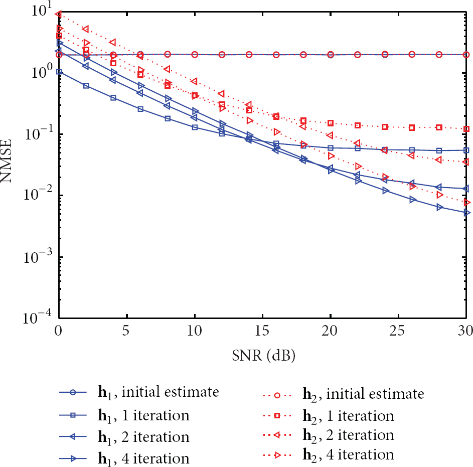
For cascaded channel estimation based on frequency domain processing at ${\text{T}}_{\mathrm{1}}$ , the NMSE performance against SNR and number of iterations are shown in Figures 2 and 3, respectively. We can see that (1) the EM-based algorithm improves the estimation accuracy by iteratively refining the cascaded channel estimates and finally approaches the corresponding maximum likelihood solutions. After 4 iterations, the NMSEs of both ${\mathit{h}}_{\mathrm{1}}$ and ${\mathit{h}}_{\mathrm{2}}$ improve a lot from the initial estimates. The improvement in the first iteration is the most significant, and the improvement in the following iterations slows down. (2) The NMSE curve of ${\mathit{h}}_{\mathrm{1}}$ estimation almost coincides with the NMSE curve of ${\mathit{h}}_{\mathrm{2}}$ estimation completely. This is because in the cascaded channel estimation, ${\mathit{h}}_{\mathrm{1}}$ and ${\mathit{h}}_{\mathrm{2}}$ are symmetrical, so the estimation performance of ${\mathit{h}}_{\mathrm{1}}$ and ${\mathit{h}}_{\mathrm{2}}$ are the same. (3) The impact of iteration number on the NMSE performance is shown in Figure 3. Here we take the estimation of ${\mathit{h}}_{\mathrm{1}}$ for example. In different SNR conditions, EM algorithm converges to the maximum likelihood solution within 10 iterations. When SNR is relatively low, the convergence of the EM algorithm is relatively fast. As SNR increases, the required iterations for convergence to the maximum likelihood solution increase accordingly.

Figure 2

Channel estimation NMSE versus SNR.

Figure 3

Channel estimation NMSE versus number of iterations.

For cascaded channel estimation based on time domain processing at ${\text{T}}_{\mathrm{1}}$ , the NMSE performance against SNR and number of iterations are shown in Figures 4 and 5, respectively. The NMSE curves demonstrate the same trend with Figures 2 and 3.

Figure 4

Channel estimation NMSE versus SNR.

Figure 5

Channel estimation NMSE versus number of iterations.

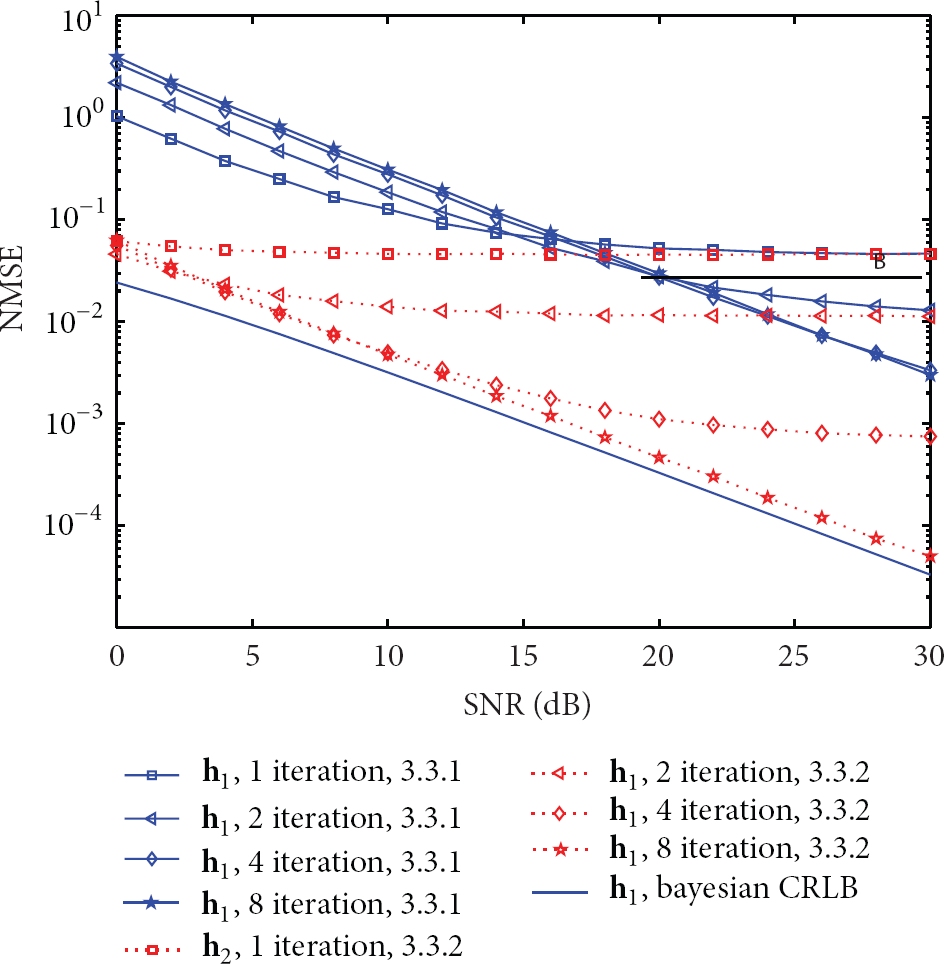
Figure 6 shows the NMSE performance comparison between the frequency domain processed estimation and the time domain processed estimation. The Bayesian CRLBs are exactly the same for the estimation of ${\mathit{h}}_{\mathrm{1}}$ and ${\mathit{h}}_{\mathrm{2}}$ , which are also plotted to measure the NMSE performance. We can see that (1) the frequency domain processed estimation converges to the maximum likelihood solution after 4 iterations, while the time domain processed estimation converges to the maximum likelihood solution after 8 iterations. When the number of iterations is the same, the estimation results of the time domain process are more accurate than the results of the frequency domain process and more close to the corresponding Bayesian CRLB.

Figure 6

Channel estimation NMSE versus SNR.

Figure 7 shows the NMSE performance comparison of the time domain processed estimation, when the power allocation between the subcarriers is not equal. The training sequences ${\mathit{d}}_{\mathrm{1}}$ and ${\mathit{d}}_{\mathrm{2}}$ are subject to the following constraints. For ${\mathit{d}}_{\mathrm{1}}$ , the power for subcarriers from 1 to 32 is halved, while the power for subcarriers from 33 to 64 increases to 1.5 times the original value. The power allocation between subcarriers is just the opposite for ${\mathit{d}}_{\mathrm{2}}$ . We can see that, compared with Figure 4, the unequal power allocation almost causes no change in the NMSE performance.

Figure 7

Channel estimation NMSE versus SNR.

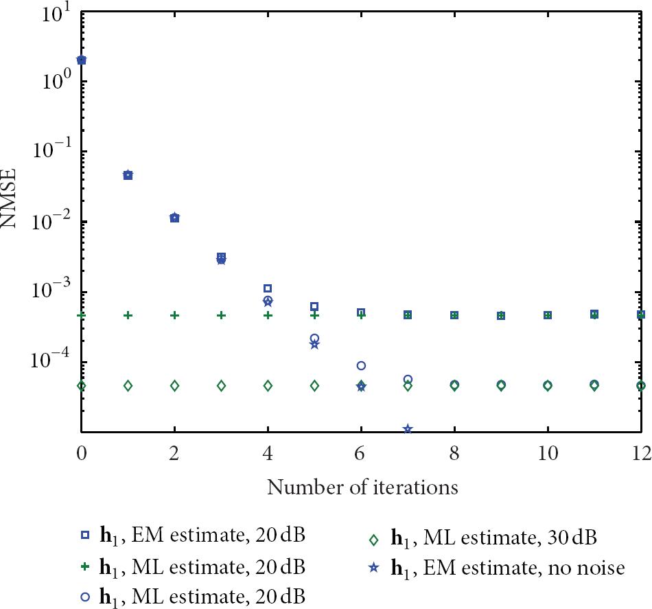
Figure 8 shows the NMSE performance of cascaded channel estimation without training sequence. We can see that the EM-based algorithm improves the estimation accuracy by iteratively refining the cascaded channel estimates. However, since ${\mathit{d}}_{\mathrm{2}}$ is unknown to the receiver at ${\text{T}}_{\mathrm{1}}$ , the convergence is slower than the counterpart in Figure 2. Moreover, the NMSE performance of ${\mathit{h}}_{\mathrm{2}}$ estimation is worse than the NMSE performance of ${\mathit{h}}_{\mathrm{1}}$ estimation, due to the inaccurate estimates of ${\mathit{d}}_{\mathrm{2}}$ . With the increase of the number of iterations, the channel estimation results become more and more accurate, the estimates of ${\mathit{d}}_{\mathrm{2}}$ becomes more and more accurate accordingly, which further improves the accuracy of channel estimation in turn.

Figure 8

Channel estimation NMSE versus SNR.

If it is possible to select a more accurate initial value to enable the EM iterations in the relay-based M2M two-way communications, the speed of convergence can be accelerated, and the performance of channel estimation can be further improved.

6. Conclusion

In this paper, we have investigated the EM-based cascaded channel estimation algorithm in relay-based M2M two-way communications, which converts the multiple-input channel estimation problem into two separate single-input channel estimation problems, leading to a considerable simplification in the computations involved and increasing the possibility of the realization of M2M communications. In the EM algorithm, the received signal at the source node is treated as the incomplete data, and the set of the two signal components from the two source nodes is modeled as the complete data. Conditioned upon the incomplete observations, the algorithm maximizes the expectation of log likelihood function defined over the complete data, by averaging over the unknown underlying parameters and using the current estimates of the cascaded channels. The algorithm iterates back and forth, using the current channel parameter estimates to decompose the received signal better and thus increase the likelihood of the next channel parameter estimates. Even in the absence of training sequence, the cascaded channel estimates can still be obtained through the iterations between the E-step and M-step. The Bayesian Cramér-Rao lower bounds have been derived under random parameters for cascaded channel estimation. The proposed method works well without channel statistical information, and the simulation demonstrates good agreement of the theoretical lower bound and the practical estimation performance.