
Abstract
The elastic stress field for multiple ellipsoidal inhomogeneous inclusions in one of two perfectly bonded semi-infinite solids subjected to external stress is investigated by the modified equivalent inclusion method. Using the general solution for the inhomogeneous inclusion in bimaterial expressed in terms of Garlekin stress vectors, the potential functions necessary to solve the problem are obtained. The elastic field induced by multiple inclusions in dissimilar media could be found from the superposition of the separate solutions of individual precipitate. The effects of the planner interface with parameters of depth from the interface and both pairs of elastic moduli and also shapes of the inclusion on the solution are given as numerical example, which is of great significance in physical applications.
1. Introduction
Using the solution of Mindlin and Cheng [1] in which the Galerkin vector was adopted and nuclei of strain were termed first, Seo and Mura [2] solved the elastic field of an ellipsoidal inclusion with uniform dilatational eigenstrains in a half-space. Eshelby [3, 4] gave the solutions for inclusion problem in an infinite isotropic solid under applied loading and the method for obtaining the solutions is called Eshelby's equivalent method. Aderogba [5] pointed out that an elastic solution for dissimilar joined half-spaces is constructed from the solution for a homogeneous whole space problem. The method for obtaining the elastic solution for a homogeneous inclusion in two joined semi-infinite solids has been developed by Yu and Sandy [6] by using the elastic solutions for the nuclei of strain in bimaterial that was solved by Yu and Sandy [7]. The expression of the analytical solution for the equivalent eigenstrains for an inhomogeneous inclusion or an inhomogeneity of arbitrary shape is obtained in terms of a system of singular integral equations as shown in Yu et al. [8]. Walpole [9] sought the problem of an inclusion located in one of two joined isotropic elastic half-spaces and evaluated the elastic strain energy that is of great significance in physical applications.
Yu and Kuang [10] discussed the thermal stresses in joined semi-infinite solids and set up the basic fracture criterion accordingly. Yu and Kuang [11] formulated method for calculation of the strain field produced by eigenstrains of one inhomogeneous inclusion located in bimaterial and the technique proposed by Moschovidis and Mura [12] was applied to extend ellipsoidal equivalency condition to the general inhomogeneity in bimaterial.
The detailed research into the problem of multiple inhomogeneous inclusions in dissimilar media under complex geometry and loading is necessary for determination of the elastic field and physical applications. The elastic interaction of multiple precipitates is an issue of practical interest in material science. Until now, although much work has been carried out as mentioned above, no general explicit exact solution of the elastic field in joined semi-infinite solids due to multiple inhomogeneous inclusions or inhomogeneities has been published to the authors' knowledge.
In the present work, the inhomogeneous precipitates are treated to have the same elastic constants of one of the two joined semi-infinite solids by application of the modified equivalent method. Under such homogeneous assumptions, the strain field can be treated as superposition of the strain field of individual precipitates and can be used to predict the alignment of precipitates. The technique of Yu et al. [8] will be used to extend Eshelby's general solution to the problem of multiple homogeneous inclusions in bimaterial. The technique of Moschovidis and Mura [12] will be used to extend Eshelby's condition of simple homogeneous inclusion to the more general inhomogeneous inclusion case. The method consists of expanding the eigenstrain, the constrained strain, and also the applied strain in Taylor series in the form of polynomials of coordinates of one global coordinate and two local coordinates. The system of singular equations is thus transformed into a system of linear algebraic equations by equating like powers of x i coordinates and comparing coefficients and then the system of algebraic equations can be solved numerically. A spherical shape was chosen for the multiple inclusions as the numerical examples for the sake of its extreme symmetry and elementary calculations that do not indeed demand any integration or solution of differential equations. The conclusions developed in this paper could be extended to other physical and geometrical phenomena, such as thermal conduction and coupled electroelastic media due to inclusions of complicated shapes such as ellipsoid and cuboid.
2. The Model of One Inhomogeneity in Joined Semi-Infinite Solid
The bimaterial is comprised of solid I (x3 ≥ 0) with Lame constants λ, μ and Poisson ratio ν and solid II (x3 ≤ 0) with Lame constants λ′, μ′ and Poisson ratio ν′ that have a common interface x3 = 0. An inhomogeneous inclusion Ω with elastic constants λ*, μ*, and ν* is located within solid I (Figure 1). Within the bounds of the infinitesimal theory of elasticity, the internal stress generated by the inclusion can be obtained by using a series of imaginary cutting, straining, and welding operations as originally given by Eshelby.

Bimaterial with the source point and its mirror point in the regions Ω and Ω′, respectively.
The imaginary procedure consists of finding a fictitious (or equivalent) homogeneous inclusion with an equivalent eigenstrain that produces identical stresses both in the inclusion and in the matrix as those due to the inhomogeneous inclusion. The equivalent eigenstrain equation for inhomogeneous inclusion in bimaterial should take the following form [10]:
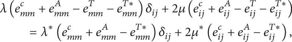
where
The goal is to find the unknown equivalent eigenstrain e ij T from the applied load e ij A and eigenstrain e ij T* in inhomogeneous inclusion. The constrained strain has the following character (see Yu and Kuang (2002b)):


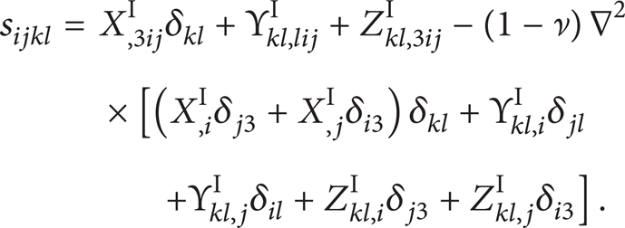
where

is a kernel with weak singularity.
Here the following relations hold:
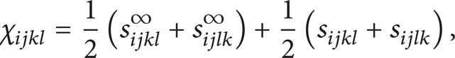

The χ ijkl is fourth rank tensor that totally has 21 components and symmetric in ij and kl. For an infinite solid that is the particular case of bimaterial, the tensor χ ijkl is degenerated to Eshelby tensor that is of wide use in micromechanics.
The integral equation given by (3) is a system of singular integral equations hard to solve with usual mathematical theory and the unknowns of equivalent eigenstrains e ij T and e ij c can be obtained by a method of successive approximations.
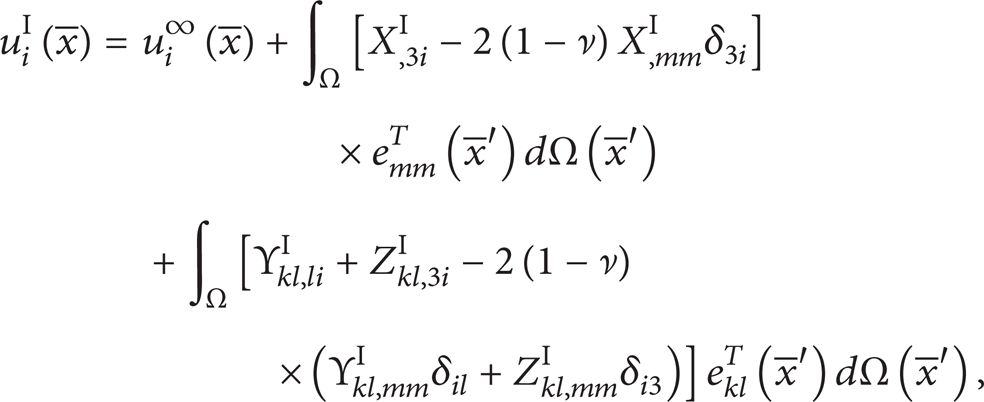
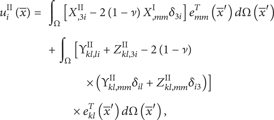
The displacements due to the inclusion Ω are the following as recorded:


where


where ν N = ν (N = 1), ν N = ν′ (N = 2).
Here g kli I and g kli II are the ith components of the Galerkin vectors at point P(x1, x2, x3) in a bimaterial in solids I and II, respectively (see [13]). Applying the method of image introduced in Yu and Kuang [10], we have for the two semi-infinite solids perfectly bonded together


where

The coefficients D and E in (11) could be obtained in the Appendix. The inclusion is situated entirely within the first phase, on the positive side of the interface. If a source point P′(x1′, x2′, x3′) is located in phase I, then its mirror point P′′ with coordinates (x1′′ = x1′, x2′′ = x2′, and x3′′ = – x3′) is in phase II and the analogous denotation will be used in the latter.
The functions R and φ are, respectively, the biharmonic potential and the harmonic potential of a unit point mass. The function θ is the logarithmic potential of a straight line with unit line density.
On substituting (9), (10a), (10b), and (11) into (8a) and (8b), the following holds:
where
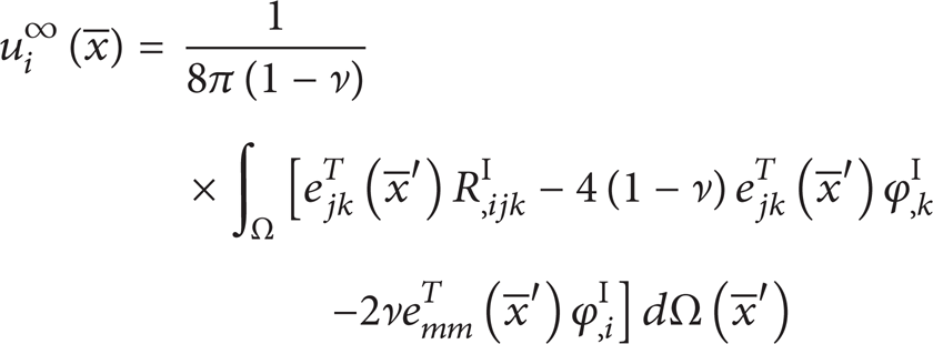
is the displacement field in an infinite solid caused by eigenstrain e ij T .
The constrained strains in the two phases are, respectively,
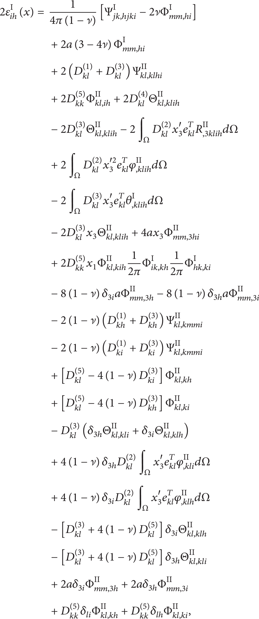

where


3. The Modified Equivalent Method
For an arbitrary precipitate within bimaterial, the constrained strain within the precipitate may not be a constant. Hence, (3) becomes intractable in its present form. Equation (3) can be modified for use with the general precipitate morphology by employing a technique firstly developed by Moschovidis and Mura [12]. Adopting some of their notation, allow the equivalent fictitious transformation strain e ij T (x) of an arbitrary shaped precipitate to be represented as a polynomial expressed in the following form:

It holds that


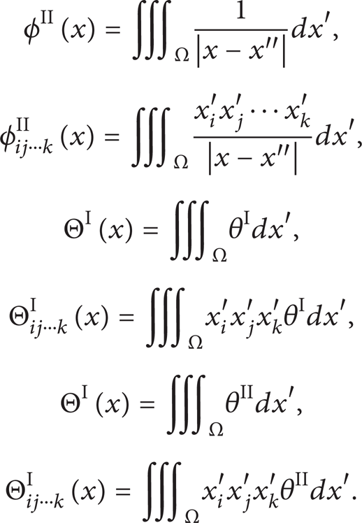
Introduce the following potential functions corresponding to ellipsoids:

The unknowns H in (17a) and (17b) are obtained in the following

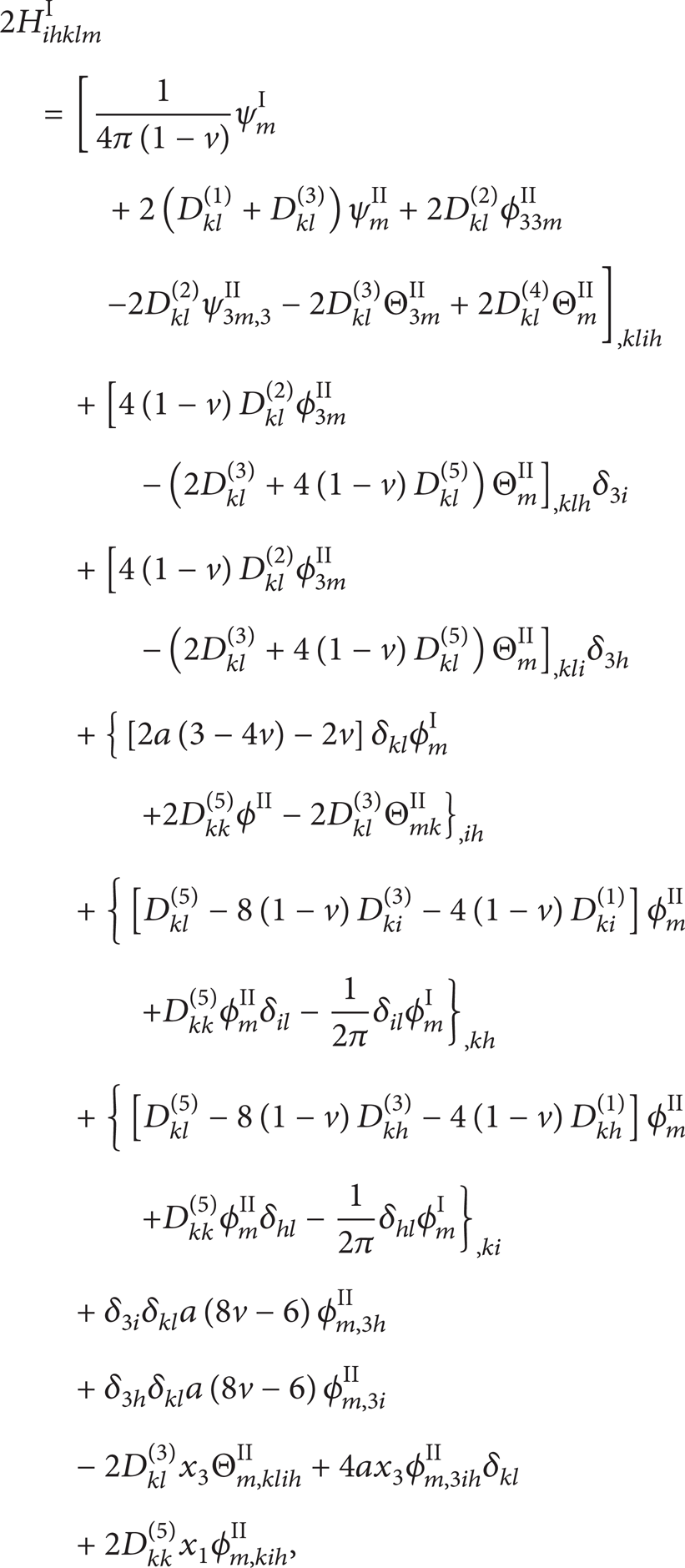


According to Dyson [14], (18) can be written as

The V-integrals above and the I-integrals are related as

where

Here a1, a2, and a3 are the three axes of the ellipsoids, respectively.
The constant λ is zero for points interior to ellipsoid and is the largest positive root of

For completeness, some explicit expressions of I (λ)-integrals for the simple geometry of ellipsoids are recorded in Mura [13]. Usually the I (λ)-integrals for general ellipsoids are much complicated to calculate and need numerical method.
The functions θI and θII are first Boussinesq potentials which are harmonic for the relevant positive and negative values of x3. The Boussinesq harmonics can be derived in turn from Newtonian ones by means of the integration. Consider

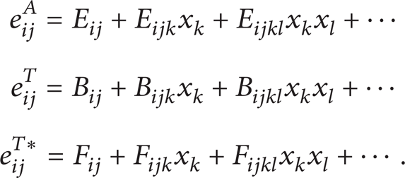
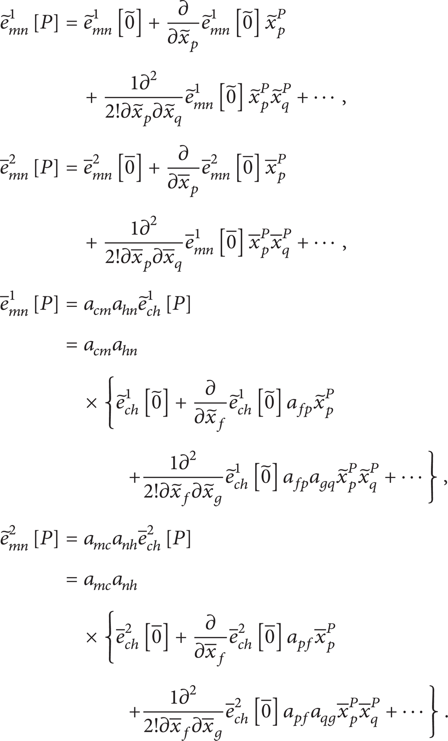
In Johnson et al. [15], by using the modified equivalency method and considering the following, we suppose that the applied load, equivalent eigenstrain, constrained strain, and the eigenstrain possessed by the inhomogeneous inclusion take the polynomial form of the global position coordinates x i as
Then

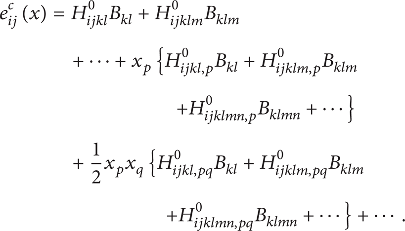
The constrained strain in (27) can be expressed in a Taylor series expanded about the origin as
4. Two Inhomogeneous Inclusions in Two Infinitely Extended Isotropic Media
Let ox1x2x3,

The global and local coordinates in biomaterial.
In this section, I and II denote the bimaterial components of phase I and phase II, respectively. The coordinates of a point P in the three systems are denoted by x
i
p
,


The equivalent eigenstrains β ij 1(x) and β ij 2(x) are expressed by


If a ij , b ij , and c ij are the transformation matrix, the following equations for the coordinate transformation hold:

The inhomogeneous inclusion may also have a given distribution of eigenstrain e ij p .
The equivalency equations are the first and second ones in (30a) and (30b). Expressing the first one in the local new system 1 in terms of the local new coordinates 1 and also the second are in the local new system 2 in terms of the local new coordinates 2, thus the equivalency equations can be written as follows:

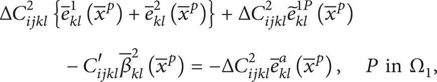
where

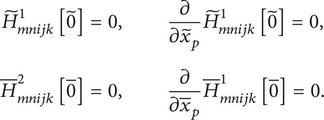
In order to satisfy the forgoing equations identically for every P in the fields, it must hold that
The induced displacement field e
ij
can be written as


On substituting (35) and (36) into (29a) and (29b), the forgoing equations are expressed in terms of the tensors
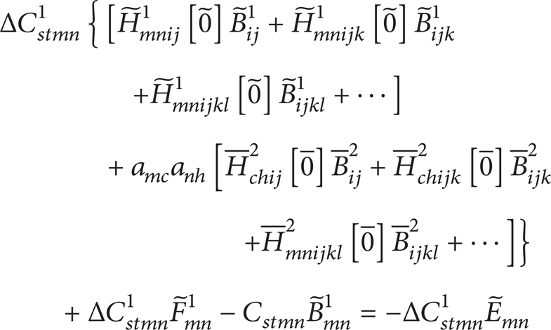


The forgoing system of algebraic equations (37a), (37b), and (37c) and (38a), (38b), and (38c) can be solved approximately if the applied field is given as a polynomial of a finite degree, for any shape of the inhomogeneous inclusions. The method of approximation is illustrated by the following examples. Let both the inhomogeneities be of ellipsoidal shape with semiaxes coinciding with the axes of the two coordinate systems, and then it holds that
Furthermore, let the applied field be given as polynomials of the first degree and let the eigenstrains be assumed as polynomials of the first degree too. The unknowns
In order to obtain accurate solution, the equivalent eigenstrains have to be assumed as polynomials of degree greater than or equal to the degree of the applied strain polynomial; the higher the degree of the eigenstrains, the better the accuracy of the solution.
If b ij and c ij are the transformation matrix, then we get the following transformation relationships of the coordinate system:

The relationship for the transformation of the constrained strain is

For material I, the eigenstrain is e ih I = e ih 1I + e ih 2I and for material II, the eigenstrain is e ih II = e ih 1II + e ih 2II.
Here e ih 1I and e ih 2I are the induced strains caused by inhomogeneous inclusions 1 and 2 in material I, respectively. Also e ih 1II and e ih 2II are the induced strains caused by inhomogeneous inclusions 1 and 2 in material II, respectively, as

Elastic field in the second inclusion caused by the first inclusion is approximated by its Taylor's expansion at the center of the second inclusion. The sum of the two elastic fields caused by individual inclusions can satisfy the required conditions for the equivalent inclusion problem at the second inclusion. A similar procedure is applied for points located in the first inclusion. The expressions for H can be found in (20a), (20b), (20c), and (20d) and the expressions for B are to be obtained from (37a), (37b), and (37c) and (38a), (38b), and (38c). So the induced strains in the two bimaterials can be resolved from (42). Then the stresses in the elastic isotropic bimaterial are, respectively,

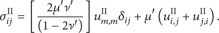
Here δ ij is the Kronecker delta and the stress inside the inhomogeneous inclusions is expressed as

where σ ij T is derived from the eigenstrain e ij T by using Hooke's law.
5. Numerical Examples
For briefness of our paper, a simple numerical example is presented to help illustrate the application of the modified equivalent method. It is assumed in Figure 3 that the inclusions are two spheres of radius a located in phase I centered at points (0,0, c1) and (0, b, c2) for c1 ≥ a and c2 ≥ a. The simplifying assumptions made here are desirable in the interest of space and for clarity of presentation of results. Relaxing these assumptions increases the complexity of calculations only nominally.

Two spherical inclusions in dissimilar media.
Stresses in (43a) and (43b) and (44) inside and outside the ellipsoidal inclusions are plotted and shown in figures in this section. To check the validity of numerical results, we have compared the present results with existing numerical solutions for one inclusion in bimaterial as obtained by Yu et al. [8]. To understand interaction effects between two inclusions, it is necessary to find out how the stress field of two inclusions behaves as a function of different geometrical parameters such as the depths c1 and c2, the location, the radii and the distance of two spheres.
Some of the calculated stresses for selected combinations of V = μ′/μ under perfectly bonded boundary conditions are illustrated in Figures 4–9. For briefness, the figures that already appeared in Yu and Kuang [10] are not drawn here, although they belong to special cases of this paper.

Stress σ33 along the ox1 axis for two spherical inclusions in bimaterial. d = 4.

Stress σ33 along the ox2 axis for two spherical inclusions in bimaterial. d = 4.

Stress σ33 along the ox3 axis for two inclusions in bimaterial. d = 4.

Stress σ33 at point (0, 0, 0) just outside the first spherical inclusion centered at (0, 0, c1) in bimaterial. d = 4.

Stress σ33 at point (0, 0, 0) just outside the first spherical inclusion in bimaterial with the radius as the parameter.

Stress σ33 at point (0, 0, 0) just outside the first spherical inclusion in bimaterial with the distance between the inclusions d as parameter.
In order to gauge the reliability of method for the potential functions in which there exists an extreme difference in elastic constants between phase I and phase II, attention is focused on the case where the parameter v equals 3 and Poisson's ratios of both materials are set to be 0.3. The dimensionless stress distributions are shown using the parameters

Here e1 = e2 = e = 1.
In an overall sense, it is found from the figures plotted that whenμ′ ≥ 10μ, the solution can be approximated by lettingμ/μ′ = 0; that is, phase II could be treated as rigid body, and when μ′ ≤ 0.1μ, the solution can be approximated by the solution for the semi-infinite solid. This conclusion is analogous to that given by Yu et al. [8].
Figures 4–7 show the effects of parameter v on the distribution of σ33 along the x1, x2, and x3 axes when the first spherical inclusion makes contact with the interface of phases I and II.
Figures 4 and 5 demonstrate the performance of stress σ33 inside the inclusion along the x1 and x2 axes, respectively. If μ′ < μ, the stress σ33 inside the inclusion increases first monotonically and then decreases and the values are always negative because the dilatational inclusion sustains the compress force due to the existence of the surrounding matrix. If μ′ = μ, the stress σ33 inside the inclusion is a negative constant, just the same as obtained long ago by Eshelby [3]. The curve (v = 0) corresponding to inclusion in a half-space has almost the same trend as that shown in Seo and Mura [2]. If μ′ > μ, the stress σ33 inside the inclusion diminishes gradually and then increases to the extremum point at the ending point of the x2 axis of the spherical inclusion.
Figure 6 demonstrates that the stress σ33 inside the inclusion is monotonically decreasing if phase II is softer than phase I, but it is monotonically increasing if phase II is harder than phase I. The distributions of stress σ33 outside the inclusion do not have much difference.
In Figure 7, it could be found out that when c1 > 1.5a, the stress component σ33 at (0,0, 0) approaches that of a semi-infinite solid with the zero value. The nearer the depth of c1, the stress is larger in its absolute value.
In Figure 8, we could find that when the first inclusion is smaller than a unit sphere, the stress will diminish monotonically as the radius of the first inclusion increases, but when it is bigger than a unit sphere, the stress will increase when phase II is softer than phase I but will continue diminishing when μ′/μ > 1.
Figure 9 illustrates the effect of distance d between the two inclusions on the stress. It is shown that if d > 4, then the stress state does not change much. If d < 4, then the larger the distance between the inclusions, the smaller will the stress be.
6. Conclusion
The solution given in this paper could be used to treat the problems of stresses and displacements in dissimilar materials arising from multiple inhomogeneous inclusions with arbitrary eigenstrains. The analysis for stress distribution is given in detail. The parametric analysis could be extended to determine a criterion for failure in bimaterial.
Our result leads to the conclusion that the method used in this paper can be utilized to predict the elastic fields resulting from arbitrarily located multiple inclusions in bimaterials reliably.
As the analytical results of this paper are of the general case, the following conclusions could be achieved accordingly.
For an ellipsoidal inclusion, when C′ ijkl = 0, ΔC ijkl 2 = 0, then (43a) and (43b) and (44) are the same as the solution obtained by Seo and Mura [2] for an ellipsoidal inclusion with pure dilatational eigenstrain in a semi-infinite solid.
When ΔC ijkl 1 = ΔC ijkl 2 = 0, then (43a) and (43b) and (44) yield the same solution as that obtained by Yu et al. [8] for a spherical homogeneous inclusion with pure dilatational eigenstrain in bimaterials.
For two ellipsoidal inhomogeneities, when C ijkl 1 = C ijkl 2 and eigenstrain e p = 0, then (43a) and (43b) and (44) give that result obtained by Moschovidis and Mura [12] for two ellipsoidal inhomogeneities under several applied stress fields in infinite solid.
For an ellipsoidal inclusion, when ΔC ijkl 2 = 0, C ijkl = C ijkl ′, then (43a) and (43b) and (44) are the same as the solutions given by Eshelby [4] for elastic inclusion and inhomogeneities in one infinite solid problem.
For multiple ellipsoidal inhomogeneous inclusion problems, when ΔC ijkl 2 = 0, (43a) and (43b), and (44) degenerate into the special solution to the problem of one inhomogeneity located in bimaterial as solved by Yu and Kuang [11].
Footnotes
Appendix
Coefficients in the elastic solution for the double forces and double forces with moment in two semi-infinite solids perfectly bonded together are [6] as follows:
where