Sage Journals: Discover world-class research

Abstract

Optimizing the path planning to reduce the time and cost is an essential consideration in modern society, and existing research has mostly concentrated on static path planning and real-time data information in vehicle navigational applications. Using dynamic path planning to adjust and update the path information in time is a challenging approach to reduce road congestion and traffic accidents. In this paper, we present a data analysis algorithm that determines an efficient dynamic path for vehicle repair-scrap sites and navigates more flexibly to avoid obstacles, where the key idea is to design the sensor wireless network that helps to obtain data from different devices. Firstly, the data processing scheme for real-time data with regional cluster and node division can be obtained from different sensor devices through the wireless senor network. Secondly, the search space and the relevant road information are restricted to a strongly connected graph. The most important strategy for an optimal solution to find the shortest path is the search method. Finally, to validate the performance of our design and algorithm, we have conducted a simulation based on necessary traffic variables. The performance simulation results show that real-time dynamic path planning can be significantly optimized using our data processing scheme.

1. Introduction

The acceleration of an automobile digitalization has led to the era of networked cars. Nowadays, China has become the largest automobile market in the world with an annual increase of 40% in car sales. There is no doubt that cars have brought convenience to our life; however, faulty cars could cause great troubles.

In order to make effective use of resources, governments at all levels in China have built sufficient repair-scrap sites to solve the problems for faulty cars. Receiving real-time information on the state of vehicles through wireless sensor network (WSN) [1, 2] and informing car owners of the closest repair-scrap sites are effective means to solve the problem of faulty cars and reduce potential traffic problems.

The key to solving this problem lies in the quantity and location of repair-scrap sites. To ensure the lowest overall costs, the average distance to the closest repair-scrap sites should be minimized. The collection and analysis of data and the issue of vehicle routing are crucial to solve this problem.

At present, automobiles mainly rely on vehicle navigation systems to receive satellite information and show the current position, driving direction, and distance from destinations on the electronic map. They choose the best driving route within the known road network range based on the shortest path principal. Currently, mature vehicle navigation systems in the market are mostly based on static path planning. When traffic accidents and road congestions occur, static path planning is unable to change routes in time. Thus, the vehicle dynamic path planning becomes a hotspot in research. With the rapid development of WSN, path search data is no longer static. Instead, data are collected, processed, and transferred through a network formed by a large number of sensor nodes distributed in a region in a self-organized manner. The sensor nodes have the characters of low-cost, low-power dissipation and the functions of perception, data processing, storage, and wireless communication [3]. With the change from static data to dynamic data, real-time information of current traffic condition can be available. The accuracy of recommended paths increases, does so the pressure on processing data; and thus, the requirement for the algorithm of data processing is more stringent.

In the issue of path optimization, the computing time increases in proportion to the increase of nodes especially in large networks. In the path optimization of large urban networks, the number and weight of nodes and edges increase dramatically; thus, the needed calculating time and real-time renewal quantity are large and can greatly affect the calculating efficiency of path optimum algorithms.

Based on the historical traffic information, combined with the current traffic information, the vehicle dynamic path planning is able to predict future traffic flow. It can adjust and update the best driving path in time to reduce traffic accidents and road congestions effectively. In recent years, the traffic status prediction becomes increasingly important to the research of vehicle navigation.

According to the understanding of specific reality, local path planning can be divided into two types: one with completely unknown environmental information and the other one with partly unknown environmental information. With the advent of the Internet, traffic information, vehicle information, and path information can be collected through the wireless sensor network. Environmental information can usually be quickly obtained so as to make global positioning which facilitates site selection.

In this paper, we propose an optimal network design model that decides the site location among vehicle repair-scrap sites. The cost of the model is minimized, proportional to the distance. The most important step for site positioning is to determine the distance.

We assume WSN, through which a large number of original data can be obtained. Preprocessing the original data according to specific demands, we can obtain data in a standard format (without abnormal data) upon which data analysis and path matching can be conducted so as to find the best path. These methods can be applications of wireless sensor networks in home area networks [4] and smart grids [5].

Depending on the existing environment and communication technologies, our efficient path planning method avoids obstacles through rectangular decomposition [6], according to the graph theory. The path planning algorithm consists of two levels: global path planning and local path planning. As to the global path planning layer, we have collected faulty sites, the location of the candidate repair centers, and the candidate scrap fields based on wireless senor network and the planning of the government.

In accordance with the scale of candidate sites, the global regional environment will be divided into several equal units by the grid method and rectangular decomposition. Local path planning is the planning of the path between two sites. According to the start site and the end site of the local area, we can choose the optimal path around obstacles in order to obtain the shortest one. We abstract the network into a graph and then find the shortest path via real-time traffic network and traffic information.

2. Related Work

The necessity of solving vehicle routing problem convinces us to analyze carefully according to given schemes. The vehicle path information is collected through wireless sensor network; then after analyzing the data, we can find the shortest path to arrive at the destination. Thus, the previous work related to this paper consists of three main aspects: data collection through wireless sensor network, data processing by graph theory, and algorithm analysis for the shortest path.

Much work has been done on wireless sensor networks. Akyildiz et al. [7] provide a review of factors that influence the design of sensor networks. It is known that, wireless sensor networks use battery-operated computing and sensing devices. Ye et al. [8] propose S-MAC, a medium access control (MAC) protocol designed for wireless sensor networks. Mainwaring et al. [9] do the in-depth study of applying wireless sensor networks to real-world habitat monitoring and other researches on wireless sensor networks [10]. Al-Karaki and Kamal [11] work on routing techniques in wireless sensor networks and data aggregation in wireless sensor networks [12]. According to these works, wireless sensor networks should care more about how to process real-time data for vehicle navigation.

On graph theory, Bryant [13] presents a new data structure to represent the Boolean functions and an associated set of manipulation algorithms. Tarjan [14] proposes an improved version of an algorithm to find the strongly connected components of a directed graph, and an algorithm to find the disconnected components of an indirect graph is presented. Some methods have been developed using graph theory [15], graph structure [16], and graph search [17–20]. Graph theory being regarded as an effective analysis tool is applied to optimization of road networks, which simplifies the problem.

In order to provide efficient vehicle path planning, a dynamic path planning method which is suitable for domestic vehicle navigation applications based on researching the dynamic road network models including arithmetic and the real-time traffic information was presented [21]. An effective transport system using global information vehicle information and communication system (VICS) and local information and communication system (IVC) was introduced [22]. The VICS, as one of the intelligent transport systems, has been developed to reduce the traffic jam; it can give real-time global information to drivers to help them find the shortest path, although the shortest path has been studied for a long time. Floyd [23] and Johnson [24] have worked on the shortest path, and there are some other related studies [25].

It can be concluded that there are two key points in the work of this paper: exploiting the vehicle navigation applications to collect real-time data information and using proper routing algorithms to minimize the total cost. As is noted above, most of these solutions are unaware of the problem that source data is so “weak” that there is only one kind of data source from GPS. Thus, in this paper we design the sensor wireless network that can obtain data from different devices such as vehicle GPS, digital camera, speed sensor, and direction sensor. As their routing algorithms cannot solve the problem of real-time path finding properly, we design a new routing algorithm based on the shortest path to deal with the real-time path finding problem.

3. Problem Definition

A minimum total cost for a repair-scrap network is needed to be built. The costs to be considered in designing repair-scrap network include construction cost and transportation cost. The following parameters and variables will be used in the proposed model:

$i \in I$ is a faulty site;

$j \in J$ is a candidate repair center;

$k \in K$ is a candidate scrap field;

$m \in M$ is the capacity of a repair center;

$h \in H$ is the capacity of a scrap field;

$a_{i}$ is the number of faulty cars at faulty site i;

$ρ_{i}$ is the proportion of faulty cars at faulty site i that is needed to be sent to repair centers;

E is the proportion of faulty cars that is needed to be scrapped after going through repair centers;

$d_{i j}$ is the distance of transporting a faulty car to repair center j from faulty site i;

$d_{i k}$ is the distance of transporting a faulty car to scrap field k from faulty site i;

$d_{j k}$ is the distance of transporting a faulty car to scrap field k from repair center j;

$C^{m}$ is the cost of building a repair center of capacity m;

$C^{h}$ is the cost of building a scrap field of capacity h;

$Θ$ the proportional coefficient.

The definitions of decision variables are as follows:

\begin{matrix} X_{j}^{m} = {\begin{cases} 1 & \begin{matrix} Build a repair center of capacity m \\ if in candidate site j \end{matrix} \\ 0 & OR, \end{cases} \\ Y_{k}^{h} = {\begin{cases} 1 & \begin{matrix} Build a scrap field of capacity h \\ if in candidate site k \end{matrix} \\ 0 & OR, \end{cases} \\ Z_{i j} = {\begin{cases} 1 & \begin{matrix} If faulty cars in faulty site i \\ are transported to repair center j \end{matrix} \\ 0 & OR, \end{cases} \\ M_{i k} = {\begin{cases} 1 & \begin{matrix} If faulty cars in faulty site \\ i are transported to scrap field k \end{matrix} \\ 0 & OR, \end{cases} \end{matrix}

(1)

$N_{j k}$ is the number of faulty cars being transported to scrap field k from repair center j.

Considering the cost of building repair centers and scrap fields and the cost of transportation, we build the following optimization model according to the features of a candidate location within the vehicle network.

The target function is

\begin{array}{l} \min C = \sum_{m} \sum_{j} C^{m} X_{j}^{m} + \sum_{h} \sum_{k} C^{h} Y_{k}^{h} + \sum_{i} \sum_{j} a_{i} ρ_{i} θ Z_{i j} d_{i j} \\ + \sum_{i} \sum_{k} a_{i} θ (1 - ρ_{i}) M_{i k} d_{i k} + \sum_{j} \sum_{k} θ N_{j k} d_{j k} . \end{array}

(2)

Formula (2) represents the minimum total cost, including the cost of building repair centers and scrap fields as well as the cost of transportation.

The following conditions should be satisfied for formula (2):

\begin{matrix} \sum_{j} Z_{i j} = 1 \forall i \in J, \end{matrix}

(3)

where

Z_{i j}

represents whether faulty car i is transported to repair center j. Formula (3) ensures that all faulty cars in all faulty sites can only be dealt with by one repair center:

\begin{matrix} \sum_{i} a_{i} ρ_{i} Z_{i j} \leq \sum_{m} {m X}_{j}^{m}, \end{matrix}

(4)

where

\sum_{m}^{} {m X}_{j}^{m}

represents the total capacity of repair center j, and

\sum_{i}^{} a_{i} ρ_{i} Z_{i j}

represents the sum of all the faulty cars in repair center j. Formula (4) ensures that the number of faulty cars transported to a repair center cannot exceed its capacity:

\begin{matrix} \sum_{i} a_{i} (1 - ρ_{i}) M_{i k} + \sum_{j} ε T_{j} N_{j k} \leq \sum_{h} m Y_{k}^{h} \forall k \in K, \end{matrix}

(5)

where

\sum_{h}^{} m Y_{k}^{h}

represents the capacity of scrap fields k.

\sum_{i}^{} a_{i} (1 - ρ_{i}) M_{i k}

represents the total number of scraped cars to scrap fields k from all faulty sites, and

\sum_{j}^{} ε T_{j} N_{j k}

represents the total number of scrapped cars to scrap fields k from all repair centers. Formula (5) represents the number of faulty cars transported to scrap fields as well as scrapped cars which cannot exceed its capacity:

\begin{matrix} \sum_{i} M_{i k} = 1 \forall k \in K, \end{matrix}

(6)

where

M_{i k}

represents whether faulty car i is transported to scrap field k. Formula (6) ensures that all faulty cars in all faulty sites can only be dealt with by one scrap field:

\begin{matrix} ε \sum_{i} a_{i} ρ_{i} Z_{i j} = \sum_{k} N_{j k} \forall j \in J, \end{matrix}

(7)

where

\sum_{k}^{} N_{j k}

represents the total number of crapped cars from repair center to scrap field j, and

ε \sum_{i}^{} a_{i} ρ_{i} Z_{i j}

represents the total number of cars from all repair centers to scrap field j. Formula (7) represents the flowing equilibrium relationship between faulty cars into repair centers and scrapped cars out of scrap fields:

\begin{matrix} \sum_{m} X_{j}^{m} \leq 1 \forall j \leq J, \end{matrix}

(8)

\begin{matrix} \sum_{h} Y_{k}^{h} \leq 1 \forall k \in K . \end{matrix}

(9)

Formula (8) represents one candidate that site that should be built as a repair center, respectively. Formula (9) represents one candidate site that should be built as a scrap field, respectively:

\begin{matrix} X_{j}^{m} \in (0, 1), Y_{k}^{h} \in (0, 1), \\ \forall j \in J, \forall m \in M, \forall h \in H, \forall k \in K, \\ Z_{i j} \in (0, 1), M_{i k} \in (0, 1), \\ \forall i \in I, \forall j \in J, \forall k \in K, \\ M_{j k} \geq 0 \forall j \in J, \forall k \in K . \end{matrix}

(10)

Formula (10) defines the constraints of decision variables

X_{j}^{m}

Y_{k}^{h}

Z_{i j}

, and

M_{i k}

This paper focuses mainly on the issue of vehicle path, as well as analyzing path d in mathematical model.

Since the objective of sites location is to find the shortest path between the two given sites in predetermined workspace, we derive a minimum total cost of a repair-scrap network for the given environmental structure that involves a number of faulty sites and a number of obstacles. In this paper, the algorithm procedure is described by rectangular decomposition, the strong connection graph, and site-to-site algorithm.

The costs to be considered include the construction cost and transportation cost, both of which are proportional to the distance. Meanwhile, the degree of crowdedness and the level of unblock for the transport path also affect path selection. According to the subjective intention of a person, you can choose the path if you want to go by the two constraints. This definition shows that the distance and the two constraints are important for the proposed global model.

4. Data Processing Scheme

Needed data are collected through wireless sensor network. Constituted by numerous cheap microsensors nodes deposited in the monitoring field, the mobile sensor network is a self-organized multihop network system. The sensor nodes have the characters of low-cost, low-power dissipation and the functions of perception, data processing, storage, and wireless communication. Data are collected through gathering, processing, and transferring the perceptive object in the area covered by network corporately.

Perceptive objects, sensor nodes, and users are three main elements of WSN. The monitoring area is the possible appearing area of the perceptive objects; perceptive objects are affairs that attract users and vary with the change of scenes. In the shortest path planning for vehicle repair-scrap sites, the perceptive objects are possible spots of faulty cars within the monitoring field. WSN usually includes sensor node, convergent node, and task management node. The convergent node has quite strong data processing and power supply ability. Normally there are one or several convergent nodes in a WSN, and a large number of common sensor nodes are distributed in the sensing field in the random or defined deployment. The sensor node is responsible for collecting information related to affairs that people are interested in, returning data along some path in the way of multihop, and finally transmitting data to task management node by the convergent node through Internet or data network with satellite. Inside sensor network, every node is not only the collector and sender of information, but also the router. Cooperating with each other, each node transmits sense data to the convergent node through multihop routing in the way of relay.

As data collection is the foundation of a research, we design the following data collection framework to obtain specific and accurate roads information.

The platform processing frame diagram (as is shown in Figure 1) consists of data collecting, data preprocessing, data analysis, and path recommendation. By gathering data through sensors, original data are obtained; after preprocessing the specific features of original data, we can get data that can be used directly for the experiment; by using algorithm of high efficiency, network data analysis and path recommendation can be realized.

Figure 1

Frame diagram of data acquisition.

To guarantee the efficiency of wireless transmission, it is inappropriate to send one datum at one time, as the sampling of the physical quantity of each node in WSN is conducted individually. Meanwhile, because of the continuity of time data, road network is divided into several sections in the design of WSN to collect original data separately. In each collection area three nodes with different functions (data node, convergent node, and task management node) are used instead of using just data node. In this way, the pressure on data transmission can be greatly reduced by simple data fusion.

As is shown in Figure 2, road network is divided into N regions, with each region consisting of 3 different nodes (data node, convergent node, and task management node). After the original data are obtained from these nodes, they will be stored in the corresponding database of each region for future research. The data obtained from sensor nodes cannot be directly used in our experiment; thus, these data should be preprocessed into the data documentation format required by specific experiments in the data procession server of each region according to different experimental requirements. After the preparation of experimental data, we search the road network in the large server according to the algorithm of this paper to recommend the best path.

Figure 2

Schematic diagram of data acquisition.

According to the features of WSN, we fractionize the examination area, or divide it based on the users' choice. Perceptive objects are crossings or paths that vehicles will pass. The examination area is the possible appearing place of perceptive object (from start to target place). Sensor node, convergent node, and task management node in the examination area upload real-time crossing information (such as no-left-turn or no-right-turn crossings, one-way street sections, and time periods in which the traffic of specific type of vehicle is closed) to Internet or satellite network, plan route with proposed algorithms, and then send back perceptive objects through convergent nodes for visual display.

Wireless sensor node and roadside access point are usually included in vehicle-based WSN in which the roadside access point plays two roles: convergent node and gateway to realize the interflow between WSN and backbone network. In the planning of the vehicle repair-scrap sites positioning, nodes in the network are vehicles loaded with road condition perception equipment. During the driving process, vehicles can collect samples of congestion and road condition along the way. At the same time, vehicles become the consumers of information, which requires the drivers to understand not only the current road condition but also road condition ahead so as to choose the best path. Roadside access point needed for the communication between related departments and vehicles also requires relaying support from sense data.

In this paper, data information is collected through WSN. Real-time information of traffic condition can be available by installing sensors like radar, camera, GPS navigator, and aerial detection in vehicles to monitor driving conditions, exhaust emission, and real-time road condition timely. And it will also bring convenience to drivers in making driving schedules.

5. Algorithm Analysis

Based on the data collected through WSN, we will design an algorithm for path planning by analyzing the established data model.

The problem to be considered is the shortest path planning for vehicle repair-scrap sites. In this paper, we restrict the geographical environment space to the strong connection graph. According to the sites and the obstacles, each site can be considered as a point whose coordinate is the site left-edge or right-edge center's coordinate. Once all points are scanned, all sites are covered. The core of the algorithm is to determine the strong connection graph in the environment firstly, mark the node based on the relationship between sites secondly, and find the shortest paths by traversing the nodes involved finally.

The planning of the vehicle repair-scrap sites positioning mainly contains four different types of sites: repair center, scrap field, faulty site, and obstacles (e.g., river, park). According to the relationship among the nodes, we need to determine the shortest path of each faulty site to every repair center and to every scrap field. Based on all the identified shortest paths, we can determine the optimal planning for the sites.

5.1. An Environment Model

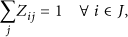
Based on the wireless senor network and the government's plan, we obtain a detailed outline of the geographical environment. The given information helps us to determine the site's position in the given environment. Then, we can mark the faulty sites, repair centers and scrap fields, and obstacles with different symbols based on their characteristics in order to establish a map of the environment as is shown in Figure 3.

Figure 3

Partially geographical environment.

5.2. A Rectangular Model

In this paper, the known grid map is used to build each site and obstacle into a rectangular model as is shown in Figure 4. All sites and obstacles are divided into various rectangles with different length and width. The definite means are as follows: (1)

find the minimum x value for each site, taking all obstacles into consideration. If more than one grid point has the minimum x value, then find the minimum y value for the grid point and mark it as $M (x_{1}, y_{1})$ ;

(2)

find the maximum x value for each site and obstacle. If more than one grid point has the maximum x value, then find the maximum y value for the grid point and mark it as $N (x_{2}, y_{2})$ ;

(3)

each site or obstacle is represented as a rectangle whose two diagonal end points are defined by the M and N.

Figure 4

A rectangular model and sites identity.

5.3. Modeling the Paths around Obstacles

Firstly, we define the concept of the line segments and the nodes for a strong connection graph.

Let R be an $m * n$ uniform grid graph that consists of a set of grid nodes ${(x, y) ∣ x$ and y are integers such that $1 \leq x \leq n, 1 \leq y \leq m}$ and grid edges connecting grid nodes. The length of grid edges connecting adjacent nodes in R is assumed to be 1.

Let $S = {S_{1}, S_{2}, \dots, S_{p}}$ be a set of mutually disjoint sites with boundaries on R. Each rectangle in S is a site.

Let $B = {B_{1}, B_{2}, \dots, B_{q}}$ be a set of mutually disjoint obstacles with boundaries on R. Each rectangle in B is an obstacle.

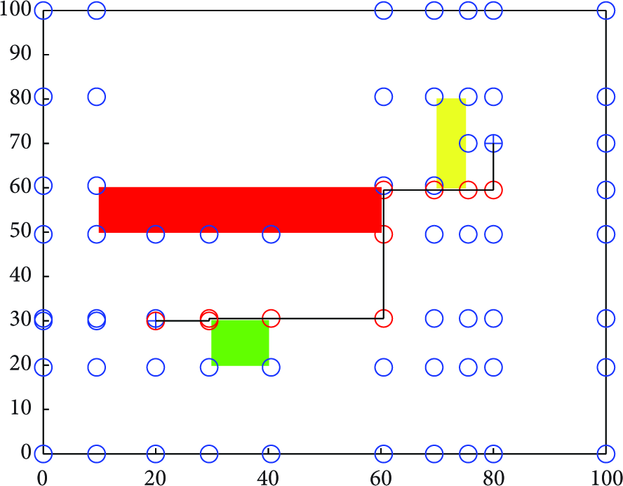
Let G denote a partial grid of R that consists of grid nodes which are not contained in the interior of any obstacle in B or any site in S and grid edges that are not incident to interior grid nodes of any obstacle in B or any site in S as is shown in Figure 5.

Figure 5

An environment model.

5.3.1. Line Segments

Each obstacle is represented as a rectangle. In order to get the shortest path from the start point to the target point, we need to construct a connection graph $G_{c}$ . The first step is to determine line segment L, as finding line segments is an important step.

Each site or obstacle rectangle has four vertices that are corresponding to the four vertices located in the upper left corner, the upper right corner, the lower right corner, and the lower left corner of the site. Let $V = {V_{1}, V_{2}, \dots, V_{p}}$ be a vertex set which consists of four vertices of each site and obstacle, start point and target point on R. In this paper, we define that the start point is one of four vertices, and s is closer to the target point t than others. Meanwhile, the target point t is one of four vertices and t is closer to the start point s than others we have decided. The line segment L is decided according to the algorithm. Figure 6 is the diagram of line segments.

Figure 6

The flow diagram of line segments search.

Step 1.

In the environment map R, let $L (R)$ be the set of line segments that form the boundaries of R.

Step 2.

We find any vertex $V_{i} (x, y)$ from vertex set V and draw the line segment in parallel with the y-axis. According to the x-axis coordinate, the sites in the space are sorted. If x is between the abscissa of the sites, and the y-axis parallel line through the point A intersects with the site, then the site is marked. And if x is not between the abscissa of the sites, let the site be marked as 0.

Step 3.

Let the line segment be in parallel with y-axis. If it is marked as 0, the line segment from $[x, 0]$ to $[x, 100]$ will be completed through A and is parallel to the y-axis. If it is marked, we need to identify the segment of the upper endpoint and the lower endpoint. Let ordinate $y 1$ of the upper endpoint $(x, y 1)$ be the minimum value of the y-coordinate by upward line parallel to the y-axis and through the point A when the first encounters a site. Let ordinate $y 2$ of the lower endpoint $(x, y 2)$ be the maximum value of the y-coordinate by downward line parallel to the y-axis and through the point A when the first encounters a site.

Step 4.

We find any vertex $V_{i} (x, y)$ from vertex set V, and draw the line segment in parallel with the x-axis. According to the y-axis coordinate, the sites in the space are sorted. If y is between the ordinate of the sites, the x-axis parallel line through the point A intersects with the site, and the site is marked. If y is not between the ordinate of the sites, let the site be marked as 0.

Step 5.

Let the line segment be in parallel with x-axis. If it is marked as 0, the line segment from $[0, y]$ to $[100, y]$ can be completed through A and parallel to the x-axis. If it is marked, we need to identify the segment of the left endpoint and the right endpoint. Let ordinate $x 1$ of the left endpoint $(x 1, y)$ be the maximum value of the x-coordinate by left line parallel to the x-axis and through the point A when the first encounters a site. Let ordinate $x 2$ of the right endpoint $(x 2, y)$ be the minimum value of the x-coordinate by right line parallel to the x-axis and through the point A when the first encounters a site.

Step 6.

If the vertex set V is null, the line segment search is completed. The line segment set is as follows $L = L (R) + L (X) + L (Y)$ ; Otherwise, return to Step 2.

Based on the above algorithm, we can decide the final line segments. For example, the line segments are shown in Figure 7.

Figure 7

Search the line segments.

5.3.2. Connection Graph

After finding the set of edges, we need to search the intersection point between the edges. Let these intersection points, start point, and target point be composed of a set of nodes. The pseudocode of generate connection graph is shown in Algorithm 1.

Algorithm 1: The initialization of the graph.

lineRec X add edge of figure

lineRec Y add edge of figure

lineRec X add DrawSegment(StartPoint) . Xsegment

lineRec X add DrawSegment(TargetPoint) . Xsegment

lineRec Y add DrawSegment(StartPoint) . Ysegment

lineRec Y add DrawSegment(TargetPoint) . Ysegment

for all barrier in BarrierPosition

for four conners of barrier

lineRec X add DrawSegment(conner) . Xsegment

lineRec $Y$ add DrawSegment(conner) . Ysegment

end

for all segment Xsegment in lineRec X

for all segment Ysegment in lineRec Y

crossPointRec add polyxpoly(Xsegment, Ysegment)

end

sortrows crossPointRec //sort the Point, and get all Points finished

//the important function—DrawSegment

function DrawSegment

sort BarrierPosition by X

get minY and maxY between x = X · x and all BarrierPosition

lineSegment X = [x, x, minY, maxY]

sort BarrierPosition by Y

get minX and maxX between y = Y · y and all BarrierPosition

lineSegment Y = [minX, maxX, y, $y$ ]

return lineSegment X and lineSegment Y

end

// The initialization of graph

for all Point point $x$ in crossPointRec

for four direction of point $x$

get the nearest Point and draw line

end

At first, it is necessary to find the relationship between these nodes in the set, for example, the intersection point which is closed to the next intersection point in the direction of X-axis and Y-axis. Through these nodes and the relations between these nodes, we abstract the whole environment into a strong connected graph as is shown in Figure 8.

Figure 8

The strong connected graph.

5.3.3. The Definition of the Shortest Path

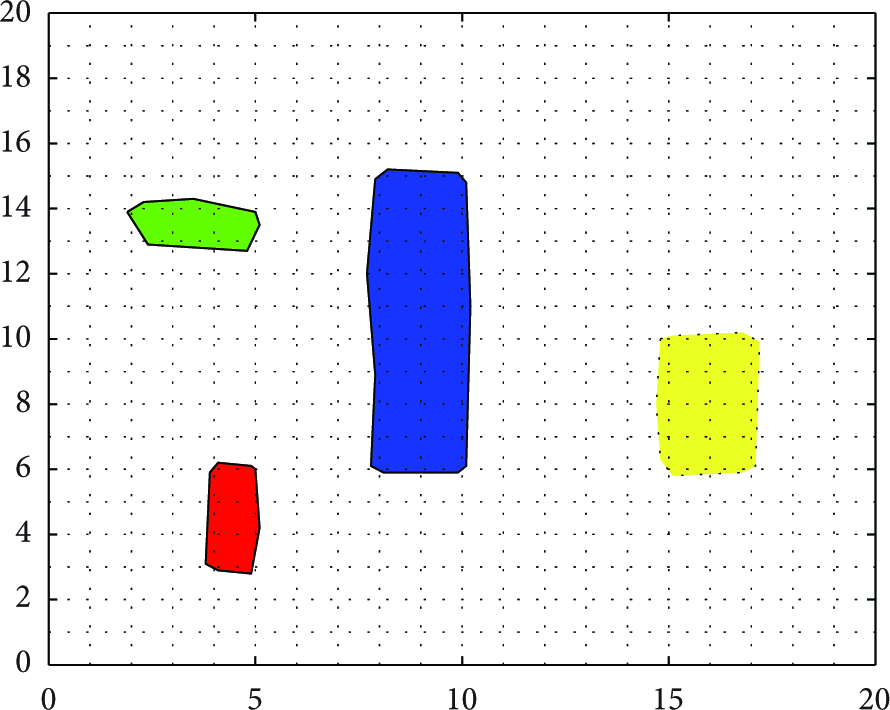
In the paper, the start point s and the target point t are faint. We define the Manhattan distance $M (s, t)$ between s and t. Let Q be any obstacle-avoiding path from s to t. The detour number $d (Q)$ is defined as the total number of nodes on Q that are directed away from t. The length of Q is $M (s, t) + 2 d (Q)$ . Q is a shortest path if and only if $d (Q)$ is minimized among all paths connecting s and t.

G is a strong connection graph for s and t. According to the coordinates of the corner points of R and obstacles in B, and a given pair of the start and target points, G can be used to find the optimal path. Let s, t be the start and target point, respectively, and v, u be any point in the shortest path, respectively. A direction assigned to an edge $(u, v)$ and the direction is from u to v. We define the detour length of $(u \to v)$ with respect to target node t denoted by $d u (u \to v)$ as shown in Figure 9. Let l be the line passing through t and perpendicular to $u \to v$ .

\begin{array}{l} d u (u ⟶ v) \\ = {\begin{cases} 0 & \begin{array}{l} if u and v are on the same side of l \\ and u is further from l than v; \end{array} \\ the length of u ⟶ v & \begin{array}{l} if u and v are on the same side of l \\ and u is closer to l than v; \end{array} \\ the length of w ⟶ v & if l intersects u ⟶ v at w . \end{cases} \end{array}

(11)

Figure 9

The definition of edge.

The detour length of a node u with respect to a source node s and a target node t, denoted by $σ (u)$ , is the sum of the detour lengths of all directed edges in any directed shortest path from s to u in G. Let P be a shortest path from s to t in G. The length of P is equal to $M (s, t) + 2 σ (t)$ .

5.3.4. The Shortest Path Algorithm

After having a clear definition of the shortest path, we can begin to search the shortest path from the start point to the target point with the space. In this section, the shortest path algorithm of site-to-site will be introduced pseudocode is shown in Algorithm 2.

Algorithm 2: The shortest path algorithm.

init VISITED set, CANDIDATES set, Point i(0-length)

add NowPoint into CANDIDATES set

while CANDIDATES set not empty

add NowPoint into VISITED set

del NowPoint from CANDIDATES set

NowPoint.visited = true

for four directions of NowPoint

NextPoint = NowPoint.direction

if NextPoint.visited = false

add NextPoint into CANDIDATES set

if DU(NowPoint) + dis(NowPoint,NextPoint) < DU(NextPoint)

DU(NextPoint) = DU(NowPoint) + dis(NowPoint,NextPoint)

Parent(NextPoint) = NowPoint

end

if CANDIDATES set is empty

break

end

set first point of CANDIDATES set as NowPoint

End

// Inverted Sequence

set TargetPoint as NowPoint

NextPoint = Parent(NowPoint)

while NextPoint not null

Draw(NowPoint,NextPoint)

NowPoint = NextPoint

NextPoint = Parent(NowPoint)

end

From the start point s, the algorithm generates graph G by points and edges, the points in the graph G are divided into two point subsets named as VISITED and CANDIDATES. Assume $DU$ is the shortest path from the start point s to any arbitrary point (set u as the point name) in the connected graph G.

In the space, the way shown in Figure 10 to find out the shortest path is as follows.

Figure 10

The flow diagram of the shortest path algorithm.

Step 1.

First, assume that the subset $V I S I T E D = \emptyset$ and the set of points defined as CANDIDATES that wait to be accessed are empty, which means that all points have not been accessed by default. Then, the $DU$ value of all points is initialized to be infinite, and the parent point is empty by default.

Step 2.

Add point s into the subset of $V I S I T E D$ and claim that point s has been accessed. Then, choose the first waiting point as the current point, which belongs to the subset of CANDIDATES and is nearest to point s.

Step 3.

Access the four “Next Points” that are near to the current point in turn and calculate the $DU$ value between s and each one of the four points. If the sum of the value of current point and the value calculated from the current point to Next Point is below the value of “Next Point,” update the value of “Next Point” as well as the parent point; otherwise, nothing is done.

Step 4.

Set the first point in the subset of CANDIDATES as Next Point, update the subset of VISITED, add the Next Point to the subset of VISITED, mark the Next Point as accessed, delete the Next Point in the subset of CANDIDATES, and add the unaccessed points near the Next Point to the subset of CANDIDATES.

Step 5.

Search in the CANDIDATES to continue finding the “Next Point” waiting to be accessed skip to Step 3 to continue. Therefore, this loop will not end until the current point reaches the last node in the CANDIDATES and the $DU$ value of each node has been calculated. The next step is to choose a path from the start point s to the target point t.

Step 6.

Setting the target point as the current point, we can find the parent point of the target point (denoted as the “Next Point”) in order to connect the current point with the “Next Point.”

Step 7.

The “Next Point” is denoted as the current point and then skips to Step 6 to continue execution. The cycle will not end until the “Next Point” meets the start point.

The simple example is shown in Figures 11, 12, and 13.

Figure 11

From the start point to search “Next Point.”

Figure 12

The shortest path.

Figure 13

Search the shortest path.

5.3.5. Congestion Weight Variables

In the above algorithmic model, we take $DU$ , the distance between the start point s to the target point t, into account when choosing the shortest path. Then the shortest path between points is decided when the $DU$ comes to its minimum.

As regarded to the practical urban traffic, the road congestion and time-phrased differences of one-way or two-way streets should be estimated. We express congestion as W (weight), the shortest distance between points as $DU$ , and the degree of priority as a%, which leads to the choice of the shortest path as follows: $L = a % \times DU + (1 - a %) W$ . $DU$ and W are equal magnitudes.

If $a = 50$ , it means that the congestion weight is as important as distance, and they have the same degree of priority. (1) If the two distances are the same, we can tell from L that the best passing path is when the congestion weights are at its minimum (Figure 14). (2) If the two congestion weight are the same, we can reach the best passing path from L when the distance $DU$ is at its minimum. (3) If both the distance $DU$ and the congestion weight are different, then through the calculation of L, the smallest minimum L is the best path.

Figure 14

Best path chosen when congestion weight is as important as distance.

According to Figure 14, the distances from the start point s to the target point t are the same through A, B, or C. Thus, the path can be decided just by comparing the congestion weight W of these three paths, $W_{A} = 128$ , $W_{B} = 120$ , and $W_{C} = 136$ , so the best travel path is path A, the red one.

If $a > 50$ , the distance $DU$ is more important than the congestion weight. Then, under that condition the driver does not take time as the first priority and is not willing to burn oil for further trip; then, he can chose to wait and stick to the shorter path, the smallest minimum of L.

Figure 15 shows the highest priority of distance $DU$ between the start point s to the target point t through path A, B, and C. Therefore, the best path can be decided by comparing the distance $DU$ of these three paths and then calculating the minimum L. In the given example, the distance is the smallest one, so the red path A is the best travel path.

Figure 15

Best path choosing when distance is more important.

If $a < 50$ , it refers that congestion weight W is more important than distance $DU$ , which means that the driver takes time as the first priority and is willing to steer clearly of the congestion road to avoid time consumption; then, the smallest minimum L is the best path.

According to Figure 16, the highest priority is the weight W from the start point s to the target point through path A, B, and C. As a result, comparing the weight W of these three paths and then calculating the smallest minimum L will lead to the best path. In this given example, $W_{A} = 128$ , $W_{B} = 120$ , and $W_{C} = 136$ , the blue path B is the best one.

Figure 16

Best path chosen when congestion weight is more important.

5.3.6. Variables of One-Way or Two-Way Road

There are many one-way roads and two-way roads in urban traffic. One-way road means that vehicles travel from entrance on one side of the road and can only exit from the other side of the road, and usually there is a sign illustrating no entrance to exit; whereas two-way road refers to the road that you can enter and exit from both sides of the road freely, usually it has two lanes, four lanes, or six lanes. Some two-way roads are timed to remit the traffic pressure. In bustling parts of the city or locations that are easily congested, one-way roads and two-way roads are often restricted by time period.

As is presented in Figure 17, the red path is the shortest path in this environmental space with the assumption that all paths are passable. However, in reality, many paths are changing between one-way road and two-way road by times. For instance, from 7:00 am to 9:00 am, and from 5:00 pm to 7:00 pm roads in front of hospitals (yellow building) are one-way roads, restricting motor vehicles except buses to travel from east to west. As a result, during these two periods, the blue path is the best path for motor passengers.

Figure 17

Best path choosing in one-way road and two-way road.

6. A Simulation Study

In order to validate the arrangement of WSN, the necessity of preprocessing, and the correctness of path search algorithm in this paper the following experiment is designed.

Figure 18 compares the use of bandwidths among three WSN arrangements (original, divide region, and divide region and node) that vary with the number of sensors.

Figure 18

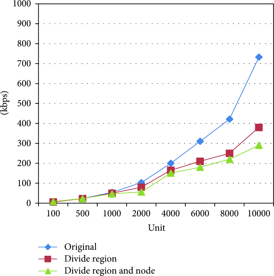
Comparison between three WSN.

From the experimental results, we can see that the bandwidth usages of the WSN arrangements are almost the same when the number of sensors is small. The bandwidth of original WSN arrangement is rather small; however, it increases sharply with the increase of sensors. The bandwidth of divide region WSN arrangement increases slowly, while for divide region and node arrangement, it increases at the slowest speed. Thus, we can see that the WSN designed in this paper can be well adapted to the transportation field using a large number of sensors.

Figure 19 shows a comparison diagram of path-searching time by using original data and preprocessed data. The horizontal axis represents the size of data, which ranges from 200 GB to 1000 GB. The vertical axis represents time spending, which is measured in seconds.

Figure 19

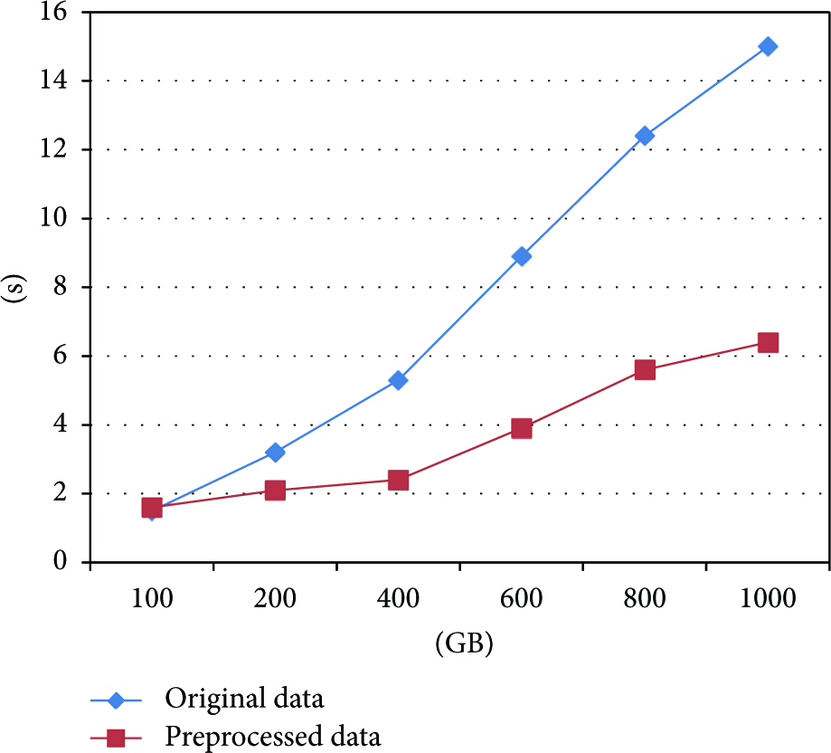
Comparison of path-searching times when using the original data versus preprocessed data.

It is obvious that using original data to search paths takes longer time than using preprocessed data. Path-searching time of original data is more than 10 seconds, which seriously affects users' experience. The preprocessed data takes less than 6 seconds in path finding which can satisfy users' demand. So preprocessed data is proved to be a right measure since path finding efficiency as well as users' experience is greatly improved in this way.

Based on divide region and node WSN arrangement, and the preprocessing of original data, we use the algorithm to find path.

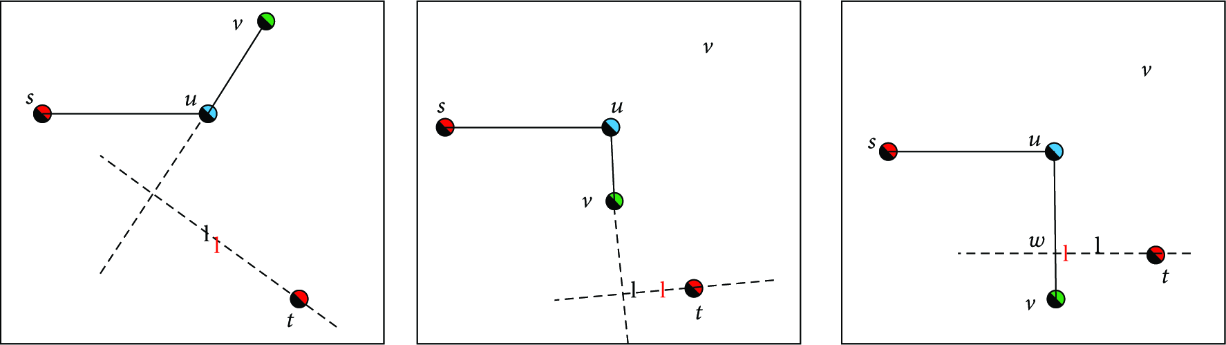
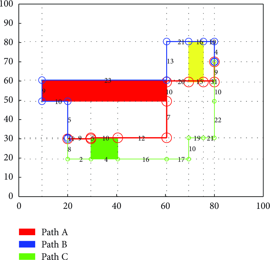
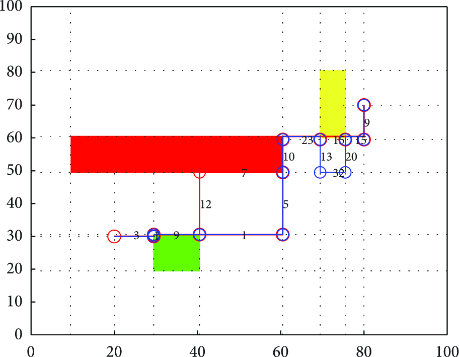
Through the practical environment of traffic network and real-time traffic, we abstract the environmental space into graphic. Then, by using the algorithm of the shortest path between points in the graph, we generate an example to test the validity of this algorithm. In this example, repair centers, scrap fields, faulty sites, and obstacles are generated from sensor devices. 20 places of faulty sites and their coordinates, quantity as well as the proportion of the failed vehicles going to repair centers or scrap fields are also generated from the sensor devices. We now assume that there are 6 repair centers and 3 scrap fields with the given coordinates, and the capacities of repair centers and scrap fields are different. Based on the above algorithm for the shortest path between points, we use MATLAB 7.0 to complete some simulated experiments. Since the algorithm is random in some way, we run the example ten times and come up with the shortest path between points that avoid obstacles, as is shown in Figure 20.

Figure 20

Result of vehicle routing problem.

Figure 20 shows that if the urban traffic network was taken into account and the path already settled, vehicles have to follow the rules of the path. There are many paths between two points. The start point and the target point have been defined by WSN, for example, the green node and red node. According to Section 5, the algorithm cares only for the shortest path between the two points rather than the start point or target point. We use the shortest path algorithm between points in accordance with transport expanse, length of path, the capacity of the points, and the degree of congestion of the roads to get the best transport path, which is illustrated in the graph. The result of the calculation presents that, on the basis of the urban traffic network, we can analyze and generate the best path information according to the information of point capacity and traffic condition gathered through the wireless sensor network. Then, drivers can choose a travel path from these best path information. If the algorithm accuracy of the solution is ensured, it will assist drivers to a great extent. Meanwhile, it is also applicable and easy to popularize.

7. Conclusion

Finding the best path that takes the shortest time is the key to a path recommendation system. This paper has proposed an algorithm based on WSN to solve the problem.

The data used in this paper are self-defined and collected through WSN. Since there are a large number of sensors in WSN, the paper proposes the following design to reduce the pressure on network bandwidth: divide the road network into several regions, while each of them has an independent server for data preprocessing to reduce pressure on the path search server. Meanwhile, the nodes in each region are divided into three types: data, convergence, and task management nodes. Data collected by adjacent nodes are sent to convergent nodes, and we just need to transmit data of convergent nodes in the network. Task management nodes are used to distribute different sensor nodes to obtain data of different types.

The original data are preprocessed into the standard format needed in the experiments. Using the proposed “site-to-site” graph algorithm and combining historical traffic information and real-time traffic information, the best path search can be conducted timely to ensure an optimal route.

Combined with historical as well as current traffic information, the algorithm can be recommended as the best path that existing recommendation algorithms cannot reach. Much work remains to be done for further improvement, such as to optimize the algorithm efficiency, to reduce the calculation interval, to experiment with more varieties of data, and to verify the correctness of this algorithm more comprehensively.

References

Mao

Z. F.

Nan

G. F.

M. Q.

A dynamic pricing scheme for congestion game in wireless machine-to-machine networks

International Journal of Distributed Sensor Networks 2012 2012 9

10.1155/2012/840391

840391

Nan

G. F.

Shi

G. X.

Mao

Z. F.

M. Q.

CDSWS: coverage-guaranteed distributed sleep/wake scheduling for wireless sensor networks

EURASIP Journal on Wireless Communications and Networking 2012 2012 1 14

Doherty

Pister

K. S. J.

El Ghaoui

Convex position estimation in wireless sensor networks

Proceedings of the 20th Annual Joint Conference of the IEEE Computer and Communications Societies

April 2001

Anchorage, Alaska, USA

1655 1663

2-s2.0-0035013232

Zhang

Xie

Yao

Xiao

Guizani

Home M2M networks: architectures, standards, and QoS improvement

IEEE Communications Magazine 2011 49 4 44 52

2-s2.0-79953778099

10.1109/MCOM.2011.5741145

Zhang

Nekovee

Liu

Xie

Gjessing

Cognitive machine-to-machine communications: visions and potentials for the smart grid

IEEE Network Magazine 2012 26 3 6 13

Tian

Liu

Feng

Zhu

Complete coverage of known space—rectangular decomposition

Chinese Journal of Mechanical Engineering 2004 40 10 56 61

2-s2.0-10644280100

Akyildiz

I. F.

Sankarasubramaniam

Cayirci

Wireless sensor networks: a survey

Computer Networks 2002 38 4 393 422

2-s2.0-0037086890

10.1016/S1389-1286(01)00302-4

Heidemann

Estrin

An energy-efficient MAC protocol for wireless sensor networks

Proceedings of the IEEE Infocom

June 2002

1567 1576

2-s2.0-0036343658

Mainwaring

Polastre

Szewczyk

Culler

Anderson

Wireless sensor networks for habitat monitoring

Proceedings of the 1st ACM International Workshop on Wireless Sensor Networks and Applications (WSNA '02)

September 2002

88 97

2-s2.0-0036986465

10.

Heidemann

Silva

Intanagonwiwat

Building efficient wireless sensor networks with low-level naming

Operating Systems Review 2001 35 5 146 159

11.

Al-Karaki

J. N.

Kamal

A. E.

Routing techniques in wireless sensor networks: a survey

IEEE Wireless Communications 2004 11 6 6 28

2-s2.0-11144277843

10.1109/MWC.2004.1368893

12.

Krishnamachari

Estrin

Wicker

The impact of data aggregation in wireless sensor networks

Proceedings of the International Conference on Distributed Computing Systems Workshop (ICDCS '02)

2002

575 578

13.

Bryant

R. E.

Graph-based algorithms for boolean function manipulation

IEEE Transactions on Computers 1986 35 8 677 691

2-s2.0-0022769976

14.

Tarjan

R. E.

Depth-first search and linear graph algorithms

Siam Journal on Computing 1972 1 2 146 160

15.

Seymour

Schrijver

Diestel

Graph theory

Oberwolfach Reports 2005 135 183

16.

Broder

Kumar

Maghoul

Raghavan

Rajagopalan

Stata

Tomkins

Wiener

Graph structure in the Web

Computer Networks 2000 33 1–6 309 320

2-s2.0-0033721503

10.1016/S1389-1286(00)00083-9

17.

Garey

M. R.

Johnson

D. S.

Stockmeyer

Some simplified NP-complete graph problems

Theoretical Computer Science 1976 1 3 237 267

2-s2.0-30244473678

18.

Battista

G. D.

Eades

Tamassia

Tollis

I. G.

Algorithms for drawing graphs: an annotated bibliography

Computational Geometry 1994 4 5 235 282

2-s2.0-43949160006

19.

Hopcroft

J. E.

Tarjan

R. E.

Dividing a graph into triconnected components

Siam Journal on Computing 1973 2 3 135 158

20.

Gansner

Koutsofios

North

K. P.

Technique for drawing directed graphs

IEEE Transactions on Software Engineering 1993 19 3 214 230

2-s2.0-0027553807

10.1109/32.221135

21.

Sun

Zhai

Zhan

Dynamic path planning techniques based on real time traffic information

Control&Automation 2007 23 3–8 177 178

22.

Fukuda

Takefuji

Ikemoto

Hasegawa

Dynamical path-planning for vehicles based on global traffic information and communication

Proceedings of the International Conference on Intelligent Transportation (ITSC '02)

2002

538 543

23.

Floyd

R. W.

Algorithm 97: shortest path

Communications of the ACM 1962 5 6 345

24.

Johnson

D. B.

Efficient algorithms for shortest paths in sparse networks

Journal of the ACM 1977 24 1 1 13

25.

Schorr

On shortest paths in polyhedral spaces

Proceedings of the ACM Symposium on Theory of Computing (STOC '84)

1984

144 153

Data Processing and Algorithm Analysis of Vehicle Path Planning Based on Wireless Sensor Network

Abstract

1. Introduction

2. Related Work

3. Problem Definition

4. Data Processing Scheme

5. Algorithm Analysis

5.1. An Environment Model

5.2. A Rectangular Model

5.3. Modeling the Paths around Obstacles

5.3.1. Line Segments

Step 1.

Step 2.

Step 3.

Step 4.

Step 5.

Step 6.

5.3.2. Connection Graph

Algorithm 1: The initialization of the graph.

5.3.3. The Definition of the Shortest Path

5.3.4. The Shortest Path Algorithm

Algorithm 2: The shortest path algorithm.

Step 1.

Step 2.

Step 3.

Step 4.

Step 5.

Step 6.

Step 7.

5.3.5. Congestion Weight Variables

5.3.6. Variables of One-Way or Two-Way Road

6. A Simulation Study

7. Conclusion

References