Self-Stabilizing TDMA Algorithms for Dynamic Wireless Ad Hoc Networks

Abstract

In dynamic wireless ad hoc networks (DynWANs), autonomous computing devices set up a network for the communication needs of the moment. These networks require the implementation of a medium access control (MAC) layer. We consider MAC protocols for DynWANs that need to be autonomous and robust as well as have high bandwidth utilization, high predictability degree of bandwidth allocation, and low communication delay in the presence of frequent topological changes to the communication network. Recent studies have shown that existing implementations cannot guarantee the necessary satisfaction of these timing requirements. We propose a self-stabilizing MAC algorithm for DynWANs that guarantees a short convergence period, and by that, it can facilitate the satisfaction of severe timing requirements, such as the above. Besides the contribution in the algorithmic front of research, we expect that our proposal can enable quicker adoption by practitioners and faster deployment of DynWANs that are subject changes in the network topology.

1. Introduction

Dynamic wireless ad hoc networks (DynWANs) are autonomous and self-organizing systems where computing devices require networking applications when a fixed network infrastructure is not available or not preferred to be used. In these cases, computing devices may set up a short-lived network for the communication needs of the moment, also known as an ad hoc network. Ad hoc networks are based on wireless communications that require implementation of a medium access control (MAC) layer. We consider MAC protocols for DynWANs that need to be autonomous and robust and have high bandwidth utilization, a high predictability degree of bandwidth allocation, and low communication delay [1] in the presence of frequent changes to the communication network topology. Existing implementations cannot guarantee the necessary satisfaction of timing requirements [2, 3]. This work proposes an algorithmic design for self-stabilizing MAC protocols that guarantees a short convergence period and, by that, can facilitate the satisfaction of severe timing requirements. The proposed algorithm possesses a greater degree of predictability, while maintaining low communication delays and high throughput.

The dynamic and difficult-to-predict nature of wireless ad hoc networks give rise to many fault tolerance issues that requires efficient solutions. DynWANs, for example, are subject to transient faults due to hardware/software temporal malfunctions or short-lived violations of the assumed settings for modeling the location of the mobile nodes. Fault tolerant systems that are self-stabilizing [4] can recover after the occurrence of transient faults, which can cause an arbitrary corruption of the system state (so long as the program's code is still intact), or the model of dynamic networks in which communication links and nodes may fail and recover during normal operation [5]. The proof of self-stabilization requires convergence from an arbitrary starting system state. Moreover, once the system has converged and followed its specifications, it is required to do so forever. The self-stabilization design criteria liberate the application designer from dealing with low-level complications, such as bandwidth allocation in the presence of topology changes, and provide an important level of abstraction. Consequently, the application design can easily focus on its task and knowledge-driven aspects.

The IEEE 802.11 standard is widely used in wireless communications. Nonetheless, the research field of MAC protocols is very active and requires further investigation. In fact, the IEEE 802.11 amendment, IEEE 802.11p, for wireless access in vehicular environments (WAVE), has just being published. It was shown that the standard's existing implementations cannot guarantee channel access before a finite deadline [2, 3]. Therefore, applications with severe timing requirements cannot predictably meet their deadlines, for example, safety-critical applications for vehicular systems.

ALOHAnet and its synchronized version slotted ALOHA [6] are pioneering wireless systems that employ a strategy of “random access.” Time division multiple access (TDMA) [7] is another early approach, where nodes transmit one after the other, each using its own timeslot, say, according to a defined schedule. Radio transmission analysis in ad hoc networks [8] and relocation analysis of mobile nodes [9] show that there are scenarios in which MAC algorithms that employ a scheduled access strategy have lower throughput than algorithms that follow the random access strategy. However, the scheduled approach offers greater predictability of bandwidth allocation and communication delay, which can facilitate fairness [10] and energy conservation [11].

Our design choices have basic radio technology in mind, whilst aiming at satisfying applications that have severe timing requirements. We consider TDMA frames with fixed number of fixed-length timeslots. The design choice of TDMA frames with fixed-length radio time fits well applications that have severe delay requirements. By avoiding the division of fixed-length frames into timeslots of non-equal length, as in [10, 12], we take into consideration the specifications of basic radio technology.

In the context of the previous design choices, there are two well-known approaches for dealing with contention (timeslot exhaustion): $(1)$ employing policies for administering message priority (for meeting timing requirements while maintaining high bandwidth utilization, such as [13]) or $(2)$ adjusting the nodes’ individual transmission signal strength or carrier sense threshold [14]. The former approach is widely accepted and adopted by the IEEE 802.11p standard, whereas the latter has only been evaluated via computer simulations. The proposed algorithm facilitates the implementation of both of the previous approaches. We consider implementation details of the standard approach in Section 7.

For the sake of presentation simplicity, we start by considering a single priority MAC protocol and base the timeslot allocation on vertex coloring, before considering multipriority implementation in Section 7. The proposed algorithm allocates timeslots to a number of nearby transmitters, that is, a number that is bounded by the TDMA frame size, whereas nonallocated transmitters receive busy channel indications. The analysis considers saturated situations in which the node degree in the message collision graph is smaller than the TDMA frame size. As explained previously, this analysis assumption does not restrict the number of concurrent transmitters when implementing the proposed MAC algorithm.

1.1. Related Work

We are not the first to propose a MAC algorithm for DynWANs that follows the TDMA's scheduled approach. STDMA [15] and Viqar and Welch [16] consider global navigation satellite system -based scheduling (GNSS) [17] according to the nodes’ geographical position and their trajectories. Autonomous systems cannot depend on GNSS services, because they are not always available, or preferred not to be used, due to their cost. Arbitrarily long failure of signal loss can occur in underground parking lots and road tunnels. We propose a self-stabilizing TDMA algorithm that does not require GNSS accessibility or knowledge about the node trajectories. Rather, it considers an underlying self-stabilizing local pulse synchronization, such as [18, 19], which can be used for TDMA alignment; details appear in [18].

When using collision detection at the receiving side [14, 15, 20–22], it is up to the receiving side to notify the sender about collisions via another round of collision-prone transmissions, say, by using frame information (FI) payload fields that include T entries, where T is the TDMA frame size. Thus far, the study of FI-based protocols has considered stochastic resolution of message collision via computer network simulation [15, 20, 22–25]. Simulations are also used for evaluating the heuristics of MS-ALOHA [14] for dealing with contention (timeslot exhaustion) by adjusting the nodes’ individual transmission signal strength and/or carrier sense threshold. We do not consider lengthy frame information (FI) fields, which significantly increase the control information overhead, and yet we provide provable guarantee regarding the convergence time. Further analysis validation of the proposed algorithm via simulations and testbed implementation can be found in Section 8, and respectively, in [18].

The proposed algorithm does not consider collision detection mechanisms that are based on signal processing or hardware support, as in [26]. Rather, it employs a variation of a well-known strategy for eventually avoiding concurrent transmissions among neighbors. This strategy allows the sending side to eventually observe the existence of interfering transmissions. Before sending, the sender waits for a random duration while performing a clear channel assessment using basic radio technology (details appear in Section 3).

There are several MAC algorithms that are based on clear channel assessment. A recent example, [12], focuses on fair bandwidth allocation for single-hop-distance broadcasting while basing the interference model on discrete graphs. The authors do not consider self-stabilization. This work also considers clear channel assessment. However, we employ a strategy of random transmission delay in a way that allows the recipients to notice, in a probabilistic manner, prospective transmissions. We show that after a small number of rounds, the system is able to use the previous strategy for allocating the network bandwidth for single-hop-distance broadcasting when basing the interference model on discrete graphs. Further mitigation efforts of transmission pathologies, such as hidden terminal phenomena when unicast are considered, can be taken, for example, self-stabilizing two-hop-distance vertex coloring [27], equalizing transmission power, and coding-based methods [28], to name a few.

An abstract MAC layer was specified for DynWANs in [29]. The authors mention algorithms that can satisfy their specifications. However, they do not consider predictability.

Local algorithms [30, 31] consider both theoretical and practical aspects of MAC algorithms ([32] and references therein) and the related problem of clock synchronization; see [33] and references therein. For example, the first partly-asynchronous self-organizing local algorithm for vertex coloring in wireless ad hoc networks is presented in [34]. However, this line currently does not consider dynamic networks and predictable bandwidth allocation.

Two examples of self-stabilizing TDMA algorithms are presented in [10, 35]. The algorithms are based on vertex-coloring and the authors consider (nondynamic) ad hoc networks. Recomputation and floating output techniques ([4], Section 2.8) are used for converting deterministic local algorithms to self-stabilization in [36]. The authors focus on problems that are related to MAC algorithms. However, deterministic MAC algorithms are known to be inefficient in their bandwidth allocation when the topology of the communication network can change frequently [9]. There are several other proposals related to self-stabilizing MAC algorithms for sensor networks, for example, [37–40]; however, none of them consider dynamic networks, and their frame control information is quite extensive.

The MAC algorithms in [9, 18, 41, 42] have no proof that they are self-stabilizing. The authors of [9] present a MAC algorithm that uses convergence from a random starting state (inspired by self-stabilization). In [18, 41, 42], the authors use computer network simulators for evaluating self-⋆ MAC algorithms.

1.2. Our Contribution

This work proposes a self-stabilizing MAC algorithm that demonstrates rapid convergence without the extensive use of frame control information. Our analysis shows that the algorithm facilitates the satisfaction of severe timing requirements for DynWANs.

We start by considering transient faults and topological changes to the communication network, that is, demonstrating self-stabilization in Theorem 2. We then turn to focus on bounding the algorithm's convergence time after an arbitrary and unbounded finite sequence of transient faults and changes to the network topology. Theorem 3 shows that the expected local convergence time is brief and bounds it in (7). Theorem 7 formulates the expected global convergence time in (21). Moreover, for a given probability, the global convergence time is calculated in (22).

For discussion (Section 8), we point out the algorithm's ability to facilitate the satisfaction of severe timing requirements for DynWANs. Moreover, the analysis conclusions explain that when allowing merely a small fraction of the bandwidth to be spent on frame control information and when considering any given probability to converge within a bounded time, the proposed algorithm demonstrates a low dependency degree on the number of nodes in the network (as depicted by Figures 2 and 3).

We note that some of the proof details appear in the Appendix for the sake of presentation simplicity.

2. Preliminaries

The system consists of a set, P, of N anonymous communicating entities, which we call nodes. Denote every node $p_i\in P$ with a unique index, i.

2.1. Synchronization

Each node has fine-grained, real-time clock hardware. We assume that the MAC protocol is invoked periodically by synchronous (common) pulse that aligns the starting time of the TDMA frame. This can be based, for example, on TDMA alignment algorithms [18], GPS [44], or a distributed pulse synchronization algorithm [19]. The term (broadcasting) timeslot refers to the period between two consecutive common pulses, $t_x$ and $t_{x+\mathrm{1}}$ , such that $t_{x+\mathrm{1}}=(t_x\mathrm{mod}T)+\mathrm{1}$ , where T is a predefined constant named the frame size. Throughout the paper, we assume that $T\ge \mathrm{2}$ . In our pseudocode, we use the event timeslot $(t)$ that is triggered by the common pulse. We assume that the timeslots are aligned as well.

2.2. Communications and Interferences

At any instance of time, the ability of any pair of nodes to communicate is defined by the set, $N_i\subseteq P$ , of (direct) neighbors that node $p_i\in P$ can communicate with directly. Wireless transmissions are subject to interferences (collisions). We consider the potential of the nodes to interfere with each other's communications. The interference model in this paper is based on discrete graphs.

The set ${𝒩}_i\supseteq N_i$ is the set of nodes that may interfere with $p_i$ 's communications when any nonempty subset of them, $I\subseteq {𝒩}_i:I\ne \varnothing$ , transmits concurrently with $p_i$ . We call ${𝒩}_i$ the (extended) neighborhood of node $p_i\in P$ , and $d_i=|{𝒩}_i|$ is named the (extended) degree of node $p_i$ . We assume that at any time, for any pair of nodes, $p_i,p_j\in P$ ; it holds that $p_j\in {𝒩}_i$ implies that $p_i\in {𝒩}_j$ . Given a particular instance of time, we define the (interference) graph as $G:=(P,E)$ , where $E:={\cup }_{i\in P}\{(p_i,p_j):p_j\in {𝒩}_i\}$ represents the interference relationships among nodes.

2.3. Communication Schemes

We consider (basic technology of) radio units that raise the event $\text{carrier}\_\text{sense}()$ when they detect that the received energy levels have reached a threshold in which the radio unit is expected to succeed in carrier locking; see [45]. Timeslots allow the transmission of $\text{DATA}$ packets using the primitives of $\text{transmit}()$ and $\text{receive}()$ after fetching ( $\text{MAC}\_\text{fetch}()$ ) a new packet from the upper layer, and respectively, before delivering ( $\text{MAC}\_\text{deliver}()$ ) the packet to the upper layer. A beacon is a short packet that includes no data load, rather the timing of the event $\text{carrier}\_\text{sense}()$ is the delivered information [12]. We assume that every node $p_i\in P$ that invokes the operation $\text{transmit}()$ causes the event $\text{carrier}\_\text{sense}()$ to be raised by its neighbors, $p_j\in {𝒩}_i$ , within the exposure time, ε. Before the transmission of the $\text{DATA}$ packet in timeslot t, our communication scheme uses beacons for signaling the node's intention to transmit a $\text{DATA}$ packet within t; see Figure 1.

Figure 1

An example of TDMA frame, with three timeslots and three listening/signaling periods of size ε (signal exposure time). Each timeslot has a constant number, $MaxRnd=\mathrm{4}$ , of listening/signaling periods in which beacons can be transmitted. The duration of each listening/signaling period is ε (signal exposure time); the period during which a beacon that is sent by node $p_i\in P$ is transmitted and raises the ca received by all neighbors $p_j\in {𝒩}_i$ . Namely, the period between $p_i$ 's transmission and $p_j$ 's rise of the $\text{carrier}\_\text{sense}()$ event.

Figure 2

Numerical validation of Theorem 7's bound on the network-wise convergence time. We compare the bound, $P(t_{\max }<k)=(\mathrm{1}-(\mathrm{1}-q{)}^k{)}^N$ , with the numerical results, which consider random geometric graphs in which the nodes are randomly placed on the unit square. The charts considers $N\in \{\mathrm{500,2500,5000}\}$ nodes (from left to right). All experiments considered $\mathrm{2}$ listening/signaling periods, interference range of $\mathrm{0.1}/\sqrt{(N/\mathrm{500})}$ , which result in an average extended degree of $\mathrm{15}$ , $d_i/T=\mathrm{1}$ on average, and $q_i=\mathrm{1}/\mathrm{4}$ .

Figure 3

Contour plot of (22) for $s=d/T=\mathrm{1}$ . Contour charts [50] present two parameter functions, for example, the convergence time function, $k(n,N)$ presented in (22). Contour lines in Figure 3 connect values of $k(n,N)$ that are the same (see the text tags along the line). When N nodes attempt to access the medium, the convergence time, 𝒮 (cf. the contour lines), is stable in the presence of a growing number, n, of listening/signaling periods.

2.4. System Settings

We consider the interleaving model [4]. Every node, $p_i\in P$ , executes a program that is a sequence of atomic steps. The state $s{t}_i$ of a node $p_i$ consists of the value of all the variables of the node (including messages in transit for $p_i$ ). Variables are associated with individual node states by using the subscript notation, that is, $va{r}_i$ is the value of variable $var$ in $p_i$ 's state. The term configuration is used for a tuple of the form $(G,\{s{t}_i{\}}_{i=\mathrm{1}}^N)$ , where G is the (interference) graph, and $\{s{t}_i{\}}_{i=\mathrm{1}}^N$ are the nodes’ states (including the set of all incoming communications). An execution (run) $R:=(c(\mathrm{0}),c(\mathrm{1}),\dots )$ is an unbounded sequence of system configurations $c(x)$ , such that each configuration $c(x+\mathrm{1})$ (except the initial configuration $c(\mathrm{0})$ ) is obtained from the preceding configuration $c(x)$ by the execution of steps, $\{a_i(x){\}}_{p_i\in P}$ , taken by all nodes.

Let τ (task) be a specification (predicate) set and $LE$ a set of all executions that satisfy task τ. Let us consider TDMA-based MAC protocols for which the task ${\tau }_{\text{TDMA}}$ requires that every node has its own broadcasting timeslot that is unique within its neighborhood. We note that ${\tau }_{\text{TDMA}}$ 's requirements are obviously satisfiable when the ratio between the extended degree and the frame size is less than one; that is, there is no timeslot exhaustion when for all $p_i\in P:\mathrm{1}⪇T/d_i$ . Therefore, the studied task also deals with timeslot exhaustion by delivering busy channel indications, ⊥, to the nodes for which there were no timeslot left. We define $L{E}_{\text{TDMA}}$ to be the set of legal executions, R, for which $\text{for}\mathrm{\hspace{0.17em}\hspace{0.17em}}\text{all}\hspace{0.17em}\hspace{0.17em}{p}_i\in P:(((s_i\in [\mathrm{0},T-\mathrm{1}])\wedge (p_j\in {𝒩}_i))\Rightarrow s_i\ne s_j)\vee (s_i=\hspace{0.17em}\perp \hspace{0.17em}\Rightarrow \text{for}\mathrm{\hspace{0.17em}\hspace{0.17em}}\text{all}\mathrm{\hspace{0.17em}\hspace{0.17em}}t\in [\mathrm{0},T-\mathrm{1}]\hspace{0.17em}\exists p_j\in {𝒩}_i:s_j=t)$ holds in all of R's configurations.

We say that configuration $c_{\text{safe}}$ is safe if there is an execution $R\in LE$ , such that $c_{\text{safe}}$ is R's starting configuration. Let R be an execution and $c\in R$ its arbitrary starting configuration. We say that R  converges with respect to τ if within a bounded number of steps from c, the system reaches a safe configuration $c_{\text{safe}}$ . The closure property requires that $R\in LE$ , for any execution, R, that starts form $c_{\text{safe}}$ . An algorithm is said to be self-stabilizing if it satisfies both the convergence and the closure properties.

We describe execution R as an unbounded number of concatenated finite sequences of configurations. The finite sequence, $R(x)=(c_{{\mathrm{0}}^{}}^{{\mathrm{\hspace{0.17em}\hspace{0.17em}}}_{}}(x),\dots c_{{T-\mathrm{1}}^{}}^{{\mathrm{\hspace{0.17em}\hspace{0.17em}}}_{}}(x))$ , $x>\mathrm{0}$ , is a broadcasting round if $(1)$ configuration $c_{{\mathrm{0}}^{}}^{{\mathrm{\hspace{0.17em}\hspace{0.17em}}}_{}}(x)$ has a clock value, t, of $\mathrm{0}$ and immediately follows a configuration in which the clock value is $T-\mathrm{1}$ , and $(2)$ configuration $c_{{T-\mathrm{1}}^{}}^{{\mathrm{\hspace{0.17em}\hspace{0.17em}}}_{}}(x)$ has a clock value of $T-\mathrm{1}$ and immediately precedes a configuration in which the clock value is $\mathrm{0}$ .

3. Algorithm Description

The proposed MAC algorithm periodically performs clear channel assessments. It uses these assessments when informing each node about the nearby unused timeslots. The nodes use this information for selecting their broadcasting timeslots, assessing the success of their broadcasts and reselecting timeslots when needed.

The MAC algorithm in Algorithm 1 satisfies the ${\tau }_{\text{TDMA}}$ task. During the convergence period, several nodes can be assigned to the same timeslot. Namely, we may have $p_i\in P:p_j\in {𝒩}_i\wedge s_i=s_j$ . The algorithm solves such timeslot allocation conflicts by letting the nodes $p_i$ and $p_j$ go through a (listening/signaling) competition before transmitting in its broadcasting timeslot. The competition rules require each node to choose one out of $MaxRnd$ listening/signaling periods for its broadcasting timeslot; see Figure 1. This implies that among all the nodes that attempt to broadcast in the same timeslot, the ones that select the earliest listening/signaling period win this broadcasting timeslot and access the communication media. Before the winners access their timeslots, they signal to their neighbors that they won via beacon transmission. The signal is sent during their choice of listening/signaling periods; see Figure 1. When a node receives a beacon, it does not transmit during that timeslot, because it lost this (listening/signaling) competition. Instead, it randomly selects another broadcasting timeslot and competes for it on the next broadcasting round.

Algorithm 1: Self-stabilizing TDMA-based MAC algorithm, code of node $p_i$ .

        Constants, variables, macros and external functions

$(\mathrm{2})$    $MaxRnd$ (n in the proofs) : integer = bound on round number

    s :  $[\mathrm{0},T-\mathrm{1}]\cup \{\perp \}$ = next timeslot to broadcast or null, ⊥

$(\mathit{4})$   signal : boolean = trying to acquire the channel

     $unused[\mathit{0},T-\mathit{1}]$  : boolean = marking unused timeslots

$(\mathit{6})$    $unused\_set=\{k:unused[k]=\mathit{t}\mathit{r}\mathit{u}\mathit{e}\}$  : unused timeslots, macro

     $\text{MAC\_fetch()/MAC\_deliver()}$  : MAC layer interface

$(\mathit{8})$    $\text{transmit/receive/carrier\_sense}$  : communication primitives

 

$(\mathit{10})$   Upon   $\text{timeslot}$ (t)

   if   $t=\mathit{0}\wedge s$   =  ⊥  then  s   $:=$    $\text{select\_unused}$ (unused_set)

$(\mathit{12})$       ( $unused[t]$ , signal) $:=$ (true, false) (* remove stale info. *)

   if  s  ≠⊥  ∧   $t=s$   then  send $\text{(MAC\_fetch())}$

$(\mathit{14})$

        Upon   $\text{receive}$ ( $〈DATA,m〉$ )  do   $\text{MAC\_deliver}$ ( $〈m〉$ )

$(\mathit{16})$

        Function   $\text{send}$ (m) (* send message m to $p_i$ 's neighbors *)

$(\mathit{18})$       for  ((signal, k) $:=$ (true, 0); $k:=k+\mathit{1}$ ; $k\le MaxRnd$ )  do

       if  signal  then  with  probability   $\rho (k)=\mathit{1}$ /( $MaxRnd-k$ )  do

$(\mathit{20})$         $signal:=\mathit{f}\mathit{a}\mathit{l}\mathit{s}\mathit{e}$ (* quit the competition *)

    transmit( $〈BEACON〉$ ) (* try acquiring the channel *)

$(\mathit{22})$  wait  until  the end of competition round (* exposure period alignment *)

   if  s  ≠⊥  then   $\text{transmit}$ ( $〈DATA,m〉$ ) (* send the data packet *)

$(\mathit{24})$

        Upon   $\text{carrier\_sense(t)}$ (* defer transmission during t *)

$(\mathit{26})$       if   $s=t\wedge signal$   then  s   $:=$   ⊥ (* mark that the timeslot is not unique *)

   (signal, $unused[t]$ ) $:=$ (false, false) (* quit the competition *)

$(\mathit{28})$

        Function   $\text{select\_unused}(set)$ (* select an empty timeslot *)

$(\mathit{30})$       if   $set=\mathrm{\varnothing }$   then  return  ⊥  else  return   $uniform\_select(set)$

In detail, the MAC algorithm in Algorithm 1 is invoked at the start of every timeslot, t. When t is the first timeslot, the algorithm tries to allocate the broadcasting timeslot, $s_i$ , to $p_i$ (line 11) by randomly selecting a timeslot for which there is no indication to be used by its neighbors. Later, when the timeslot t becomes $p_i$ 's broadcasting timeslot, $s_i$ , the node attempts to broadcast (by calling the function $\text{send}()$ in line 13). We note that the start of timeslot t also requires the marking of t as an unused timeslot and the removal of stale information (line 12). This indication is changed when the $\text{carrier}\_\text{sense}(\text{t})$ event is raised (line 27) due to a neighbor transmission; namely, when the detected energy levels reach a threshold in which the radio unit is expected to succeed in carrier locking; see [45].

When a node attempts to broadcast, it uses the (listening/signaling) competition mechanism for deciding when to signal to its neighbors that it is about to transmit a $\text{DATA}$ packet. The competition has $MaxRnd$ rounds, and it stops as soon as the node transmits a beacon or a neighbor succeeds in signaling earlier (lines 18 to 23). We note that this signaling is handled by the $\text{carrier}\_\text{sense}(t)$ event (line 27). Moreover, beacons are not required to carry payloads or any other information that is normally stored in packet headers. They are rather used to invoke the carrier sense event in ${𝒩}_i$ .

The carrier sense in timeslot t indicates to each node that it needs to defer from transmission during t (line 25). In particular, it should stop using timeslot t for broadcasting, stop competing, and mark t as a used timeslot. Lastly, arriving DATA packets are delivered to the upper layer (line 15).

4. Correctness Proof: Outline and Notation

The proof starts by considering networks that do not change their topology and for which the ratio between the extended node degree and the frame size is less than one, that is, for all $p_i\in P:\mathrm{1}⪇T/d_i$ . (We deal with cases in which for all $p_i\in P:\mathrm{1}⪇T/d_i$ does not hold in Section 8). For these settings, we show that the MAC algorithm in Algorithm 1 is self-stabilizing with respect to task ${\tau }_{\text{TDMA}}$ (Appendicies A to B), before considering the convergence time within a single neighborhood (Section 5) and the entire neighborhood (Section 6). These convergence estimations facilitate the exploration of important properties, such as predictability, and dealing with changes in the network topology of DynWANs (Section 8).

4.1. ProofOutline

The exposition of the proof outline refers to Definition 1, which delineates the different states at which a node can be in relation to its neighbors. Definition 1 groups these states into three categories of relative states: (1)   $\text{Ready}$ to be allocated, when the node state depicts correctly its neighbor states, (2)   $\text{Obtaining}$ a timeslot, when the node is competing for one, but there is no agreement with its neighbor states, and (3)   $\text{Allocated}$ to a timeslot, when the node is the only one to be allocated to a particular timeslot in its neighborhood. The correctness proof shows that the MAC algorithm in Algorithm 1 implements ${\tau }_{\text{TDMA}}$ in a self-stabilizing manner by showing that eventually all nodes are allocated with timeslots; that is, all nodes are in the relative state $\text{Allocated}$ ; see Definition 1.

Let R be an execution of the MAC algorithm in Algorithm 1 and $R(x)$ the xth complete broadcasting round of R, where $x>\mathrm{0}$ is an integer. We simplify the presentation by using uppercase notation for the configurations, $c_{t^{}}^{{\text{name}}_{}}(x)$ , where $t\in [\mathrm{0},T-\mathrm{1}]$ is a timeslot. This notation includes the $name$ of the first event to be triggered immediately after configuration c, that is, $R(x)=(c_{{\mathrm{0}}^{}}^{{\text{timeslot}}_{}}(x),\dots c_{{T-\mathrm{1}}^{}}^{{\text{carrier}\_\text{sense}/\text{receive}}_{}}(x))$ .

Definition 1.

We say that node $p_i\in P$ is $\text{Ready}$ (to be allocated) to a timeslot in configuration $c_{{\mathrm{0}}^{}}^{{\text{timeslot}}_{}}(x)$ , if properties (1), (2), and (3) hold for node $p_i$ , but Property (4) does not. We say that $p_i$ is $\text{Obtaining}$ timeslot $s_i$ in configuration $c_{{\mathrm{0}}^{}}^{{\text{timeslot}}_{}}(x)$ , if properties (1) to (4) hold for node $p_i$ , but Property (5) does not. We say that node $p_i\in P$ is in $\text{Allocated}$ state, with respect to timeslot $s_i$ in configuration $c_{{\mathrm{0}}^{}}^{{\text{timeslot}}_{}}(x)$ , if properties (1) to (5) hold for node $p_i$ as follows:

$$\begin{array}{cc}& \mathrm{\hspace{0.17em}\hspace{0.17em}}\text{signa}{\text{l}}_i=\text{false}\end{array}$$

(1)

$$\begin{array}{cc}& \left(t\in \text{unuse}{\text{d}}_i\wedge t\ne s_i\right)⟷\left(\forall p_k\in {𝒩}_i:s_k\ne t\right)\end{array}$$

(2)

$$\begin{array}{cc}& s_i\hspace{0.17em}\ne \hspace{0.17em}\perp \vee \hspace{0.17em}\hspace{0.17em}\text{unused}\_\text{se}{\text{t}}_i\setminus \left\{s_i\right\}\ne \varnothing \end{array}$$

(3)

$$\begin{array}{cc}& s_i\hspace{0.17em}\ne \hspace{0.17em}\perp \end{array}$$

(4)

$$\begin{array}{cc}& \forall p_j\in {𝒩}_i:\left(\left(s_i\ne s_j\right)\wedge \left({\text{unused}}_j\left[s_i\right]=\text{false}\right)\right).\end{array}$$

(5)

Property (1) implies that node $p_i$ finishes any broadcast attempts within a timeslot. Properties (2) to (3) consider the case in which $p_i$ 's internal state represents correctly the timeslot allocation in its neighborhood. In particular, property (2) means that processor $p_i$ views timeslot t as an unused one if, and only if, it is indeed unused. Property (3) implies that when node $p_i$ is not using any timeslot, there is an unused timeslot at its disposal. Property (4) says that node $p_i$ is using timeslot $s_i$ . Property (5) refers to situations in which $p_i$ 's neighbors are not using $p_i$ 's timeslot during the next broadcasting round.

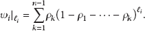
Starting from an arbitrary configuration, we show that node $p_i$ becomes $\text{Ready}$ within two broadcasting rounds (or one complete broadcasting round); see Appendix A. Then, we consider the probability, $OnlyOn{e}_i(x)$ , that a node enters the relative state $\text{Allocated}$ from either $\text{Ready}$ or $\text{Obtaining}$ ; see (6) (and Appendices B and D). Namely, (6) considers the probability that node $p_i$ is the only one to use its broadcasting timeslot in its neighborhood, where ${\rho }_k=\mathrm{1}/MaxRnd=\mathrm{1}/n$ is $p_i$ 's probability to select the kth listening/signaling period for transmitting its beacon.

Consider

$$\begin{array}{cc}& OnlyOn{e}_i\left(x\right)\ge \sum _{k=\mathrm{1}}^n‍{\rho }_k{\left(\mathrm{1}-\sum _{\ell =\mathrm{1}}^k‍{\rho }_{\ell }\right)}^{d_i/T}.\end{array}$$

(6)

Theorem 2 demonstrates self-stabilization.

Theorem 2 (self-stabilization, the proof appears in Appendix C).

The MAC algorithm in Algorithm 1 is self-stabilizing with respect to the task ${\tau }_{\text{TDMA}}$ .

Bounding the convergence time. We bound the time it takes the MAC algorithm in Algorithm 1 to converge by considering the relative states, $\text{Ready}$ , $\text{Obtaining}$ , and $\text{Allocated}$ and describe a state machine of a Markovian process. This process is used for bounding the convergence time of a single node (Section 5) and the entire network (Section 6).

In detail, given node $p_i\in P$ , its neighborhood ${𝒩}_i$ , we define a random environment of a Markov chain; see Box 1. By looking at this random environment, we can focus our analysis on $p_i$ 's relative states while avoiding probability dependencies and considering average probabilities [46]. Suppose that $p_i$ 's environment, e, is known. Theorem 3 estimates two bounds on the expectation of probability $q_i{\hspace{0.17em}|\hspace{0.17em}}_e$ , which is literally the probability $q_i$ , given that the environment is e.

Box 1: Markov chain describing $p_i$ 's relative state transitions.

We look at $p_i$ 's state transition with relation to its neighbors; see

Definition $\mathit{1}$ . The figure on the top defines $p_i$ 's relative states

as a 3-state Markov chain. The probabilities, $q_i$ , $w_i$ , $f_i$ , and $h_i$

(solid lines arrows), that node $p_i$ change its relative state depend

on its neighbor's state. For instance, $q_i$ is the probability that $p_i$

goes from the relative state $\text{Ready to Allocated.}$ It is environment-

dependent; that is, the states of $p_i$ 's neighbors are random as well.

We added the dotted edge between the state $\text{Allocated}$ and the state

$\text{Ready}$ in order to make the Markov chain irreducible and to allow

working with the invariant probability. Namely, once node $p_i$

arrives to $\text{Allocated}$ , it returns to $\text{Ready}$ with probability 1. With

this convention, we can estimate the expected time to reach the

final relative state $\text{Allocated}$ from relative state $\text{Ready}$ by the

expectation of the first hitting time of the irreducible chain [43]

In order to do that, we consider a set, ℛ, of executions of the MAC algorithm, such that each execution $R\in ℛ$ starts in a configuration, $c\in R$ , in which (I) for any node $p_j\in P$ , properties (1), (2), and (3) hold, and (II) node $p_i$ is in the relative state $\text{Ready}$ , which implies that (III) eventually, node $p_i$ arrives to the relative state $\text{Allocated}$ .

With this convention, we can add a probability 1 to transit from the relative state $\text{Allocated}$ to $\text{Ready}$ ; see the dashed line in the state machine diagram of Box 1. This allows us to estimate the expected time to reach the final relative state $\text{Allocated}$ from relative state $\text{Ready}$ by the expectation of the first hitting time of the irreducible Markov chain [43].

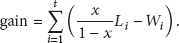
When computing the expected time for node $p_i$ to reach state $\text{Allocated}$ within its neighborhood, we see that it is sufficient to consider the lower bound of the probability $OnlyOn{e}_i(x)$ to obtain an upper bound on the expected time to convergence; see Section 5. Moreover, when considering the network convergence time, that is, the expected convergence time of all nodes in the network, we see that the most dominant parameter is the mean neighborhood size. We do that by applying the arithmetic mean versus geometric mean (AM-GM) inequality and bounding the expected network convergence time; see Section 6.

4.2. Notation

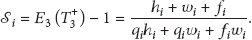
Throughout the paper, we denote the states of the Markov chain by $\{X_t{\}}_{t\ge \mathrm{0}}$ , $T_i^{+}=\min \{t>\mathrm{0}\mathrm{\hspace{0.17em}\hspace{0.17em}}\text{such}\mathrm{\hspace{0.17em}\hspace{0.17em}}\text{that}\mathrm{\hspace{0.17em}\hspace{0.17em}}{X}_t=i\}$ and $E_i(·)$ is the expectation, given that we start in relative state i, $E_i(T_i^{+})=E(T_i^{+}\hspace{0.17em}|\hspace{0.17em}{X}_{\mathrm{0}}=i)$ . In this paper, the states $\mathrm{1}$ , $\mathrm{2}$ , and $\mathrm{3}$ of the Markovian process correspond, respectively, to states $\text{Ready}$ , $\text{Obtaining}$ , and $\text{Allocated}$ and the time $t=\mathrm{0,1},\dots$ corresponds to configuration $c_{\mathrm{0}}^{\text{timeslot}}(x+t)\in R(x+t)$ , where $R(x)$ is the first complete broadcasting round in R that starts in a configuration, $c_{\mathrm{0}}^{\text{timeslot}}(x)$ , in which all nodes are in the relative state $\text{Ready}$ . For example, $E_{\mathrm{3}}(T_{\mathrm{3}}^{+})$ is the expected time to reach the $\text{Allocated}$ state.

Let $p_i\in P$ be a node for which $s_i\ne \hspace{0.17em}\perp \hspace{0.17em}\wedge \hspace{0.17em}\hspace{0.17em}\exists p_j\in {𝒩}_i:s_j=s_i$ in configuration $c_{{\mathrm{0}}^{}}^{{\text{timeslot}}_{}}(x)$ . We define $M_i(x)=\{p_j\in {𝒩}_i:s_i=s_j\}$ to be the set of $p_i$ 's (broadcasting timeslot) matching neighbors, which includes all of $p_i$ 's neighbors that, during broadcasting round $R(x)$ , are attempting to broadcast in $p_i$ 's timeslot. In our proofs, we use n as the number of listening/signaling periods, $MaxRnd$ .

5. Convergence within a Neighborhood

Theorem 3 bounds the expected time, ${𝒮}_i$ , for a node to reach the relative state $\text{Allocated}$ , and follows from Proposition 5 and (12). Note that ${𝒮}_i\le \mathrm{4}$ when the number of listening/signaling periods is $n\ge \mathrm{2}$ and considering saturated situations in which the extended node degree $d_i<T$ is smaller than the TDMA frame size. Namely, the proposed algorithm convergence with a neighborhood is brief.

Theorem 3 (local convergence).

The expected time, ${𝒮}_i$ , for node $p_i\in P$ to reach the relative state $\text{Allocated}$ satisfies (7), where n is the number of listening/signaling periods, T is the TDMA frame size, and $d_i$ is $p_i$ 's extended degree.

Consider

$$\begin{array}{cc}& {𝒮}_i\le \min \left\{{\left(\frac{\mathrm{2}n}{n-\mathrm{1}}\right)}^{d_i/T},\frac{d_i/T+\mathrm{1}}{n}{\left(\frac{n}{n-\mathrm{1}}\right)}^{d_i/T+\mathrm{1}}\right\}.\end{array}$$

(7)

We look into the transition probability among relative states by depicting the diagram of Box 1 as a homogeneous Markov chain. We estimate the diagram transition probabilities in a way that maximizes the expected time for reaching the diagram's final state, $\text{Allocated}$ . It is known that the first hitting time is given by $E_i(T_i^{+})=\mathrm{1}/{\pi }_i$ , where $\pi =({\pi }_{\mathrm{1}},{\pi }_{\mathrm{2}},{\pi }_{\mathrm{3}})$ is the invariant probability vector [43]. Let ${𝒮}_i$ be the expected time it takes node $p_i$ that starts at the relative state $\text{Ready}$ to reach $\text{Allocated}$ . It is clear that ${𝒮}_i=T_{\mathrm{3}}^{+}-\mathrm{1}$ , because $T_{\mathrm{3}}^{+}-\mathrm{1}$ is the return time of the relative state $\text{Allocated}$ . In our case, the transition matrix P is given by the following:

$$\begin{array}{cc}& P=\left(\begin{array}{ccc}\mathrm{1}-f_i-q_i& f_i& q_i\\ h_i& \mathrm{1}-h_i-w_i& w_i\\ \mathrm{1}& \mathrm{0}& \mathrm{0}\end{array}\right).\end{array}$$

(8)

The invariant probability vector π satisfying $\pi P=\pi$ is given by

$$\begin{array}{cc}& \pi =\frac{(h_i+w_i,f_i,q_i{h}_i+q_i{w}_i+f_i{w}_i)}{h_i+w_i+f_i+h_i{q}_i+q_i{w}_i+f_i{w}_i}.\end{array}$$

(9)

The estimation of the maximal expected time necessary to assign the node $p_i$ to a timeslot requires us to compute bounds on the probabilities $f_i$ , $h_i$ , $q_i$ and $w_i$ that maximize as follows

$$\begin{array}{cc}& E_{\mathrm{3}}\left(T_{\mathrm{3}}^{+}\right)=\frac{\mathrm{1}}{{\pi }_{\mathrm{3}}}=\frac{h_i+w_i+f_i+h_i{q}_i+q_i{w}_i+f_i{w}_i}{q_i{h}_i+q_i{w}_i+f_i{w}_i}.\end{array}$$

(10)

The expected time for $p_i$ to reach the relative state $\text{Allocated}$ is bounded in

$$\begin{array}{cc}& {𝒮}_i=E_{\mathrm{3}}\left(T_{\mathrm{3}}^{+}\right)-\mathrm{1}=\frac{h_i+w_i+f_i}{q_i{h}_i+q_i{w}_i+f_i{w}_i}.\end{array}$$

(11)

Equation (7) has a compact and meaningful bound for (11). We achieve that by studying the impact of the parameters T and n on the MAC algorithm in Algorithm 1. Lemma 4 and (11) imply

$$\begin{array}{cc}& {𝒮}_i\le \frac{h_i+w_i+f_i}{q_i{h}_i+q_i{w}_i+f_i{q}_i}=\frac{\mathrm{1}}{q_i}.\end{array}$$

(12)

Lemma 4.

Suppose that $n\ge \mathrm{2}$ is the number of listening/signaling periods; see line 2 of the code in Algorithm 1. Then $w_i\ge q_i$ .

Proof.

Let us consider node $p_i\in P$ that is in relative state $\text{Ready}$ . Given that $p_i$ has $v_i$ neighbors that compete for the same timeslot, the probability that $p_i$ gets allocated, $q_i{\hspace{0.17em}|\hspace{0.17em}}_{v_i}$ , is given by (13).

$$\begin{array}{cc}& q_i{\hspace{0.17em}|\hspace{0.17em}}_{v_i}=\sum _{k=\mathrm{1}}^{n-\mathrm{1}}‍{\rho }_k{\left(\mathrm{1}-{\rho }_{\mathrm{1}}-\cdots -{\rho }_k\right)}^{v_i}.\end{array}$$

(13)

Consider next that $p_i$ is in relative state $\text{Obtaining}$ , and thus, we know that $p_i$ transmitted during the preceding broadcasting round and transited from relative state $\text{Ready}$ to $\text{Obtaining}$ . Moreover, $p_i$ is using the same timeslot for the current broadcasting round. The only neighbors of $p_i$ that are using the same timeslot are the neighbors that are also in relative state $\text{Obtaining}$ and have chosen the same listening/signaling period as $p_i$ during the preceding broadcasting round. Let us denote by ${\ell }_i$ , the number of such neighbors. Given ${\ell }_i$ the probability $w_i{\hspace{0.17em}|\hspace{0.17em}}_{{\ell }_i}$ that $p_i$ is allocated to the timeslot is given by

$$\begin{array}{cc}& w_i{\hspace{0.17em}|\hspace{0.17em}}_{{\ell }_i}=\sum _{k=\mathrm{1}}^{n-\mathrm{1}}‍{\rho }_k{\left(\mathrm{1}-{\rho }_{\mathrm{1}}-\cdots -{\rho }_k\right)}^{{\ell }_i}.\end{array}$$

(14)

We have that ${\ell }_i$ is stochastically dominated by $v_i$ [47], that is, $E({\ell }_i)\le E(v_i)$ . Indeed, $v_i$ is a random variable that counts the number of neighbors that choose the same timeslot as $p_i$ , while ${\ell }_i$ counts the number of neighbors that choose the same timeslot and listening/signaling period as $p_i$ . For $n\ge \mathrm{2}$ , ${\ell }_i$ 's expected value is smaller than $v_i$ 's expected value. To conclude, we remark that expressions (13) and (14) are the same decreasing function, $f_i\to {\sum }_{k=\mathrm{1}}^{n-\mathrm{1}}‍{\rho }_k{(\mathrm{1}-{\rho }_{\mathrm{1}}-\cdots -{\rho }_k)}^{f_i}$ , that is evaluated at two different points, $v_i$ and ${\ell }_i$ , respectively. Moreover, since ${\ell }_i$ is stochastically dominated by $v_i$ , (15) holds as follows:

$$\begin{array}{cc}& w_i=E\left(w_i{\hspace{0.17em}|\hspace{0.17em}}_{{\ell }_i}\right)\ge E\left(q_i{\hspace{0.17em}|\hspace{0.17em}}_{v_i}\right)=q_i.\end{array}$$

(15)

Proposition 5 demonstrates (16) and leads us toward the proof of Theorem 3.

Proposition 5.

Let ${\rho }_i=\mathrm{1}/MaxRnd$ . Equation (16) bounds from below the probability $q_i$ ; see Appendix D of the.

Consider

$$\begin{array}{cc}& q_i\ge \max \left\{{\left(\frac{n-\mathrm{1}}{\mathrm{2}n}\right)}^{d_i/T},\frac{\mathrm{1}}{d_i/T+\mathrm{1}}{\left(\mathrm{1}-\frac{\mathrm{1}}{n}\right)}^{d_i/T+\mathrm{1}}\right\}.\end{array}$$

(16)

The first bound, $\mathrm{1}/q_i\le {(\mathrm{2}n/(n-\mathrm{1}))}^{d_i/T}$ ((7)), has a simple intuitive interpretation. Let us consider first that two nodes compete for a same timeslot. The two nodes choose independently any of the n listening/signaling periods and there are $n^{\mathrm{2}}$ different possible outcomes. Among these outcomes n correspond to the situation where the two nodes choose the same listening/signaling period and there is no winner. We then have $n^{\mathrm{2}}-n=n(n-\mathrm{1})$ outcomes that lead to a winner. There is then a probability of $n(n-\mathrm{1})/n^{\mathrm{2}}=(n-\mathrm{1})/n$ that one of the nodes wins the (listening/signaling) competition. Since the game is symmetric, the probability that $p_i$ wins is $(n-\mathrm{1})/(\mathrm{2}n)$ . The fact that we have T timeslots divides the number of competing nodes, $d_i$ , and implies that there are $d_i/T$ competing nodes for the same timeslot. If we interpret the game as a collection of $d_i/T$ independent games, where for each game $p_i$ wins with probability $(n-\mathrm{1})/(\mathrm{2}n)$ , thus, the probability $q_i$ that $p_i$ wins is ${((n-\mathrm{1})/\mathrm{2}n)}^{d_i/T}$ . The inverse of this expression gives the average time for the event to occur and is the bound by (7).

6. Network Convergence

We estimate the expected time for the entire network to reach a safe configuration in which all nodes are allocated with timeslots. The estimation is based on the number of nodes that are the earliest to signal in their broadcasting timeslot. These nodes are winners of the (listening/signaling) competition and are allocated to their chosen timeslots. However, counting only these nodes leads to underestimating the number of allocated nodes, which then results in an overestimation of the convergence time. Indeed, node $p_i\in P$ might have a neighbor $p_j\in {𝒩}_i$ that selects the earliest listening/signaling period in ${𝒩}_i$ , but $p_j$ does not transmit because one of its neighbors, $p_k\in {𝒩}_j\setminus {𝒩}_i$ , had transmitted in an earlier listening/signaling period. Our bound considers only $p_k$ while both $p_i$ and $p_k$ transmit, became $p_j$ is inhibited by $p_k$ 's beacon.

Lemma 6 shows that the assumption that the nodes are allocated independently of each other is suitable for bounding the network convergence time, 𝒮. Theorem 7 uses Lemma 6 for bounding the network convergence time, 𝒮.

In Section 5, we prove a bound on the expected time, ${𝒮}_i$ , for a single node to be allocated to a timeslot. We observe that the bound depends uniquely on the number of listening/signaling periods, n, as well as the ratio between the extended degree and the frame size, $d_i/T$ . In order to obtain a bound valid for all nodes, we bound this ratio with $x/T$ where x is as defined in Lemma 6. We note that the time needed for the allocation of timeslots to all the nodes depends on N, the total number of nodes.

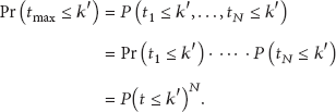
In detail, the convergence time estimation considers the (fixed and independent) bound, $q_i$ , for the probability that a node reaches the relative state $\text{Allocated}$ within a broadcasting round. Then, the convergence time, t, is a random variable with geometric probability, that is, $P(t\mathrm{\hspace{0.17em}\hspace{0.17em}}=\mathrm{\hspace{0.17em}\hspace{0.17em}}k)\mathrm{\hspace{0.17em}\hspace{0.17em}}=\mathrm{\hspace{0.17em}\hspace{0.17em}}(\mathrm{1}\mathrm{\hspace{0.17em}\hspace{0.17em}}-\mathrm{\hspace{0.17em}\hspace{0.17em}}q{)}^{k-\mathrm{1}}q$ . Let us denotes $t_{\mathrm{1}},\dots ,t_N$ the time it takes for the nodes $p_{\mathrm{1}},\dots ,p_N$ to respectively reach the relative state $\text{Allocated}$ . The convergence time, 𝒮, for all the nodes is given with $\max (\{t_{\mathrm{1}},\dots ,t_N\})$ , which depends on N.

Lemma 6.

The expected number of nodes, $E(W)$ , that win the (listening/signaling) competition after one broadcasting round satisfies (17), where $x=\mathrm{2}A/N$ , T is the number of timeslots, A the number of edges in the interference graph, G, and $N=|P|$ the number of nodes that attempt to access the communication media.

Consider

$$\begin{array}{cc}& E\left(W\right)\ge N\sum _{j=\mathrm{1}}^n‍{\rho }_j{\left(\mathrm{1}-\left({\rho }_{\mathrm{1}}+\cdots +{\rho }_j\right)\right)}^{x/T}.\end{array}$$

(17)

Proof.

The nodes that are allocated to a timeslot can previously be on relative state $\text{Ready}$ or $\text{Obtaining}$ . The probability of a transition from relative state $\text{Obtaining}$ to $\text{Allocated}$ is $w_i$ , and a transition from relative state $\text{Ready}$ to $\text{Allocated}$ is $q_i$ . As proved in Lemma 4, we always have $w_i\ge q_i$ . To bound the number of nodes that get allocated during a broadcasting round, we use the lower bound on the probability $q_i$ that a node gets allocated to a timeslot. Moreover, in the computations, we use the AM-GM bound [48], which says that if $\sum ‍b_k=\mathrm{1}$ then ${\prod }_{}‍a_k^{b_k}\le \sum ‍b_k{a}_k$ and denote by $d_i$ the number of neighbors of node $p_i$ . As proved in Proposition D.1, since there are T timeslots the number of neighbors of i that choose the same timeslot as i and compete for it is bounded by $d_i/T$ . This lemma is proved by (18), where the last line of the expression holds because ${\sum }_i‍d_i=\mathrm{2}A$ .

One has

$$\begin{array}{l}E\left(W\right)\ge E\left(\sum _{i=\mathrm{1}}^N‍{\mathrm{1}}_{|p_i\mathrm{\hspace{0.17em}\hspace{0.17em}}\text{selects}\mathrm{\hspace{0.17em}\hspace{0.17em}}\text{the}\mathrm{\hspace{0.17em}\hspace{0.17em}}\text{earliest}\mathrm{\hspace{0.17em}\hspace{0.17em}}\text{signaling}\mathrm{\hspace{0.17em}\hspace{0.17em}}\text{period}}\right)\\ \hspace{1em}\hspace{1em}\hspace{0.5em}=\sum _{i=\mathrm{1}}^N‍\left({\rho }_{\mathrm{1}}{\left(\mathrm{1}-{\rho }_{\mathrm{1}}\right)}^{d_i/T}+\cdots {\rho }_{n-\mathrm{1}}{\left(\mathrm{1}-\sum _{k=\mathrm{1}}^{n-\mathrm{1}}‍{\rho }_k\right)}^{d_i/T}\right)\\ \hspace{1em}\hspace{1em}\hspace{0.5em}=\sum _{j=\mathrm{1}}^n‍N\sum _{i=\mathrm{1}}^N‍\frac{\mathrm{1}}{N}{\rho }_j{\left(\mathrm{1}-\sum _{k=\mathrm{1}}^j‍{\rho }_k\right)}^{d_i/T}\end{array}$$

(18)

$$\begin{array}{l}\hspace{1em}\hspace{1em}\hspace{0.5em}\ge N\sum _{j=\mathrm{1}}^n‍\prod _{i=\mathrm{1}}^N‍{\rho }_j^{\mathrm{1}/N}{\left(\mathrm{1}-\sum _{k=\mathrm{1}}^j‍{\rho }_k\right)}^{d_i/NT}\\ \hspace{1em}\hspace{1em}\hspace{0.5em}=N\sum _{j=\mathrm{1}}^n‍{\rho }_j{\left(\mathrm{1}-\sum _{k=\mathrm{1}}^j‍{\rho }_k\right)}^{\left(\mathrm{1}/TN\right)\sum ‍d_i}\\ \hspace{1em}\hspace{1em}\hspace{0.5em}=N\sum _{j=\mathrm{1}}^n‍{\rho }_j{\left(\mathrm{1}-\sum _{k=\mathrm{1}}^j‍{\rho }_k\right)}^{x/T}.\end{array}$$

(19)

We note that we use the AM-GM bound to reach the 4th row of (18).

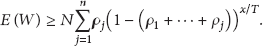
By arguments similar to the ones used in the proof of Proposition 5, we deduce that if N nodes compete, the expected number $E(W)$ of nodes that get allocated to a timeslot is lower bounded as follows:

$$\begin{array}{cc}& E\left(W\right)\ge N\max \hspace{0.17em}\left\{{\left(\frac{n-\mathrm{1}}{\mathrm{2}n}\right)}^{x/T},\frac{{\left(\left(n-\mathrm{1}\right)/n\right)}^{x/T+\mathrm{1}}}{x/T+\mathrm{1}}\right\}.\end{array}$$

(20)

Theorem 7 bounds the system convergence time. We numerically validate Theorem 7; see Figure 2. Moreover, our experiments showed that the average convergence time of the network is below the upper bound of (21).

Theorem 7 (global convergence).

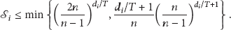
The expected number of retransmissions is smaller than ${(\mathrm{2}n/(n-\mathrm{1}))}^{d/T}-\mathrm{1}$ , where $d=\max (\{d_i:p_i\in P\})$ . Hence, one has that the expected number of broadcasting rounds, 𝒮, that guarantee that all nodes reach the relative state $\text{Allocated}$ satisfies

$$\begin{array}{cc}& 𝒮\le {\left(\frac{\mathrm{2}n}{n-\mathrm{1}}\right)}^{d/T}.\end{array}$$

(21)

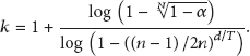
Moreover, given that there are N nodes in the network and $\alpha \in (\mathrm{0,1})$ , the network convergence time is bounded by (22) with probability $\mathrm{1}-\alpha$ .

Consider

$$\begin{array}{cc}& k=\mathrm{1}+\frac{\log \hspace{0.17em}\left(\mathrm{1}-\sqrt[N]{\mathrm{1}-\alpha }\right)}{\log \hspace{0.17em}\left(\mathrm{1}-{\left(\left(n-\mathrm{1}\right)/\mathrm{2}n\right)}^{d/T}\right)}.\end{array}$$

(22)

This means that with probability α, all nodes are allocated with timeslots in maximum k broadcasting rounds; see Figure 3.

Proof.

Theorem 3 bounds the convergence time of a particular processor; see (7). Lemma 6; see (20) $E(W)\ge N((n-\mathrm{1})/\mathrm{2}n{)}^{x/T}$ , proves that this bound is still valid if we replace the term $d_i/T$ with $x/T$ ; that is, we consider the average degree instead of the particular degree of a node. If we replace $x/T$ by $\max \{d_i\}/T$ in expression (20) we obtain a larger bound because $x/T\le \max \{d_i\}/T$ ; that is, $E(W)\ge N((n-\mathrm{1})/\mathrm{2}n{)}^{x/T}\ge N((n-\mathrm{1})/\mathrm{2}n{)}^{\max \{d_i\}/T}$ .

The bound $E(W)\ge N((n-\mathrm{1})/\mathrm{2}n{)}^{\max \{d_i\}/T}$ and the discussion in the $\mathrm{1}\text{st}$ paragraph of Section 6 show that the number of processors that are allocated during a broadcasting round is bounded by the random variable ${\sum }_{i=\mathrm{1}}^N‍z_i$ , where $z_i$ are identically and independently distributed random variables that are $\mathrm{1}$ with probability $((n-\mathrm{1})/\mathrm{2}n{)}^{\max \{d_i\}/T}$ and $\mathrm{0}$ with probability $\mathrm{1}-((n-\mathrm{1})/\mathrm{2}n{)}^{\max \{d_i\}/T}$ (the second random variable dominates the first one; see [49]). This means that we lower bound the number of processors that are allocated if we consider that they are allocated independently with probability $((n-\mathrm{1})/\mathrm{2}n{)}^{\max \{d_i\}/T}$ .

While the processors get allocated to a timeslot, the parameters $d_i$ and T change because some timeslots are no longer available (T decreases, some nodes are allocated, $d_i$ decreases). Actually the ratio becomes $(\max \{d_i\}-h_i)/(T-f_i)$ , where $h_i\ge f_i$ because if a timeslot is allocated or sensed used by processor $p_i$ , then T, the number of available timeslots decreases by $\mathrm{1}$ and $d_i$ , the number of competing nodes, must decrease at least by one since there must be at least one processor that uses the busy timeslot (there may be multiple that are in state $\text{Obtaining}$ ). Under these circumstances, we always have $\max \{d_i\}/T\ge (\max \{d_i\}-h_i)/(T-f_i)$ . Thus, we can obtain a lower bound for the expected time to reach the relative state $\text{Allocated}$ by assuming that all nodes are allocated independently with probability $x=((n-\mathrm{1})/\mathrm{2}n{)}^{\max \{d_i\}/T}$ . We simplify the following arguments by using this definition of x.

To bound the number of broadcasting rounds, we consider the following game. The bank pays 1 unit to the nodes that get in state $\text{Allocated}$ (get allocated to a timeslot) and receives $x/(\mathrm{1}-x)$ units per nodes that fail to get in state $\text{Allocated}$ . The game is fair because in each round the expected gain is $\mathrm{1}\times x-x/(\mathrm{1}-x)\times (\mathrm{1}-x)=\mathrm{0}$ . If we denote by $W_i$ the number of processors that get in state $\text{Allocated}$ during the ith broadcasting round and by $L_i$ the number of processors that fail, we have that the gain is given by (23), where t denotes the total number of rounds.

One has

$$\begin{array}{cc}& \text{gain}=\sum _{i=\mathrm{1}}^t‍\left(\frac{x}{\mathrm{1}-x}{L}_i-W_i\right).\end{array}$$

(23)

The expected gain is $\mathrm{0}$ because the game is fair ( $E(\text{gain})=\mathrm{0}$ ) and ${\sum }_{i=\mathrm{1}}^t‍W_i=N$ because eventually all the nodes get in state $\text{Allocated}$ and the bank pays $\mathrm{1}$ unit for each such processors. If we compute the expectation on both sides of (23), we then obtain

$$\begin{array}{cc}& N=\frac{x}{\mathrm{1}-x}E\left(\sum _{i=\mathrm{1}}^t‍L_i\right).\end{array}$$

(24)

We observe that $E({\sum }_{i=\mathrm{1}}^t‍L_i)$ is the expected total number of retransmissions and $E({\sum }_{i=\mathrm{1}}^t‍L_i)/N$ is the average expected number of retransmissions whose value is $(\mathrm{1}-x)/x$ . Replacing x with its expression, we obtain that the average number of retransmission is bounded by $(\mathrm{2}n/(n-\mathrm{1}){)}^{\max \{d_i\}/T}-\mathrm{1}$ , and, this leads to the bound (21).

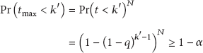
To prove the second assertion, let $t_{\mathrm{1}},\dots ,t_N$ be the convergence time of nodes $\mathrm{1},\dots ,N$ , respectively. The random variables, $t_i$ , are bound by random variables with geometric random distribution with expectation of $(\mathrm{2}n/(n-\mathrm{1}){)}^{d/T}$ , with $d=\max \{d_i:d_i\in P\}$ . We require that $t_{\max }=\max \{t_{\mathrm{1}},\dots ,t_N\}$ in order to ensure that all nodes are allocated with timeslots. The fact that the random variables, $t_i$ , are independent and identically distributed, implies (25), where t is a random geometrical random variable, that is, $\text{Pr}(t=k^{\prime })=(\mathrm{1}-q{)}^{k^{\prime }-\mathrm{1}}q$ and $\text{Pr}(t\ge k^{\prime })=(\mathrm{1}-q{)}^{k^{\prime }-\mathrm{1}}$ .

Consider

$$\begin{array}{l}\text{Pr}\left(t_{\max }\le k^{\prime }\right)=P\left(t_{\mathrm{1}}\le k^{\prime },\dots ,t_N\le k^{\prime }\right)\\ =\text{Pr}\left(t_{\mathrm{1}}\le k^{\prime }\right)·\hspace{0.17em}\cdots \hspace{0.17em}·P\left(t_N\le k^{\prime }\right)\\ =P{\left(t\le k^{\prime }\right)}^N.\end{array}$$

(25)

Which $t_{\max }\le k^{\prime }$ satisfies (26) with probability α?

One has

$$\begin{array}{l}\text{Pr}\left(t_{\max }<k^{\prime }\right)=\text{Pr}{\left(t<k^{\prime }\right)}^N\\ ={\left(\mathrm{1}-{\left(\mathrm{1}-q\right)}^{k^{\prime }-\mathrm{1}}\right)}^N\ge \mathrm{1}-\alpha \end{array}$$

(26)

By solving (26), we observe that (26) is satisfied for any $k^{\prime }\ge k$ , where k satisfies (22). This proves that, with probability $\mathrm{1}-\alpha$ , the network convergence time is bounded by (22).

7. Implementation

Existing MAC protocols offer mechanisms for dealing with contention (timeslot exhaustion) via policies for administering message priority, such as [13]. In particular, the IEEE 802.11p standard considers four priorities and techniques for facilitating their policy implementation. We explain similar techniques that can facilitate the needed mechanisms.

7.1. Prioritized Listening/Signaling Periods

We partition the sequence of listening periods, $[\mathrm{0},MaxRnd)$ , into $MaxPrt$ subsequences, $[\mathrm{0},MaxRn{d}_{\mathrm{0}}),\dots [MaxRn{d}_{MaxPrt-\mathrm{2}},MaxRn{d}_{MaxPrt-\mathrm{1}})$ , where $[MaxRn{d}_{k-\mathrm{1}},MaxRn{d}_k)$ is used only for the kth priority. For example, suppose that there are six listening/signaling periods and that nodes with the highest priority may use the first three listening/signaling periods, $[\mathrm{0,2}]$ , and nodes with the lowest priority may use the last three, $[\mathrm{3,5}]$ . In the case of two neighbors with different listening period parameters, say, $[\mathrm{0,2}]$ and $[\mathrm{3,5}]$ , that attempt to acquire the same broadcasting timeslot, the highest priority node always attempts to broadcast before the lowest priority one.

7.2. TDMA-Based Backoff

Let us consider two backoff parameters, $\text{C}{\text{W}}_{\text{start}}$ and $\text{C}{\text{W}}_{\text{end}}$ , that refer to the maximal and minimal values of the contention window. Before selecting an unused timeslot, the procedure counts a random number of unused ones. Algorithm 2 presents an implementation of the $\text{select}\_\text{unused}()$ function that facilitates backoff strategies as an alternative to the implementation presented in line 29 of Algorithm 1.

Algorithm 2: $\text{Select\_unused()}$ with TDMA-based backoff.

     Additional constants and variables

$(\mathrm{2})$          $C{W}_{start}$ and $C{W}_{end}$  : backoff parameters

       count : statically allocated variable that counts the backoff steps

  $(\mathrm{4})$

        Function   $\text{select\_unused(}$ set)

$(\mathrm{6})$         let   $rtn\_val$ = $\perp \_v\_$ // indicate busy channel (default return value)

       if   $count\le \mathrm{0}$   then   $count\leftarrow uniform\_select([C{W}_{start},C{W}_{end}])$

$(\mathrm{8})$          $count\leftarrow count$   −   $\hspace{0.17em}|\hspace{0.17em}set\hspace{0.17em}|\hspace{0.17em}$

       if   $count\le \mathrm{0}$   then   $(count,rtn\_val)\leftarrow (\mathrm{0},uniform\_select(set))$

$(\mathrm{10})$     return   $rtn\_val$

 

The statically allocated variable $count$ records the number of backoff steps that node $p_i$ takes until it reaches the zero value. Whenever the function $\text{select}\_\text{unused}()$ is invoked with $coun{t}_i=\mathrm{0}$ , node $p_i$ assigns to $coun{t}_i$ a random integer from $[\text{C}{\text{W}}_{\text{start}},\text{C}{\text{W}}_{\text{end}}]$ (cf. line 7). Whenever the value of $coun{t}_i$ is not greater than the number of unused timeslots, the returned timeslot is selected uniformly at random (cf. lines 8 to 9). Otherwise, a ⊥-value is returned after deducting the number of unused timeslots during the previous broadcasting round (cf. lines 6 and 10).

8. Discussion

Thus far, both schedule-based and nonschedule-based MAC algorithms could not consider timing requirements within a provably short recovery period that follows (arbitrary) transient faults and network topology changes. This work proposes the first self-stabilizing TDMA algorithm for DynWANs that has a provably short convergence period. Thus, the proposed algorithm possesses a greater predictability degree, whilst maintaining low communication delays and high throughput.

In this discussion, we would like to point out the algorithm's ability to facilitate the satisfaction of severe timing requirements for DynWANs by numerically validating Theorem 7. As a case study, we show that, for the considered settings of Figure 2, the global convergence time is brief and definitive. Figure 3 shows that when allowing merely a small fraction of the bandwidth to be spent on frame control information, say, three listening/signaling periods, and when considering 99% probability to convergence within a couple of dozen TDMA frames, the proposed algorithm demonstrates a low dependency degree on the number of nodes in the network even when considering 10,000 nodes.

We have implemented the proposed algorithm, extensively validated our analysis via computer simulation, and tested it on a platform with more than two dozen nodes [18]. These results indeed validate that the proposed algorithm can indeed facilitate the implementation of MAC protocols that guarantee satisfying these severe timing requirements.

The costs associated with predictable communications, say, using cellular base stations, motivate the adoption of new networking technologies, such as MANETs and VANETs. In the context of these technologies, we expect that the proposed algorithm will contribute to the development of MAC protocols with a higher predictability degree.