Optimal Management of Rechargeable Biosensors in Temperature-Sensitive Environments

Abstract

Biological sensors (biosensors, for short) are tiny wireless devices attached or implanted into the body of a human or animal to monitor and detect abnormalities and then relay data to physician or provide therapy on the spot. They are distinguished from conventional sensors by their biologically derived sensing elements and by being temperature constrained. Biosensors generate heat when they transmit their measurements and when they are recharged by electromagnetic energy. The generated heat translates to a temperature increase in the tissues surrounding the biosensors. If the temperature increase exceeds a certain threshold, the tissues might be damaged. In this paper, we discuss the problem of finding an optimal policy for operating a rechargeable biosensor inside a temperature-sensitive environment characterized by a strict maximum temperature increase constraint. This problem can be formulated as a Markov Decision Process (MDP) and solved to obtain the optimal policy which maximizes the average number of samples that can be generated by the biosensor while observing the constraint on the maximum safe temperature level. In order to handle large-size MDP models, it is shown how operating policies can be obtained using Q-learning and heuristics. Numerical and simulation results demonstrating the performance of the different policies are presented.

1. Introduction

Biosensors are tiny wireless devices attached or implanted into the body of a human or animal to monitor and detect abnormalities and then relay data to physician or provide therapy on the spot. Unlike conventional wireless sensors, biosensors are energy as well as temperature constrained. Also, their sensing elements are biological materials such as enzymes and antibodies which are integrated into transducers for producing electrical signals in response to biological reactions and changes. Biosensors are powered by either rechargeable built-in batteries or by continuously sending electric energy to them in the form of electromagnetic waves.

The use of batteries necessitates periodic recharging which can be performed using energy resulting from vibration, motion, light, and heat. However, a more mature approach is to wirelessly collect energy from a Radio Frequency (RF) source and then convert it into usable power. This approach is widely used in the industry to transfer data and power to biosensors. It is also more practical since many biosensors can be recharged simultaneously. In essence, a charging station generates a magnetic field that can convey energy through the skin. From the penetrating magnetic field, an electric voltage is produced by induction in the receiver circuit. The induced voltage is then rectified, filtered, and stabilized to run the biosensors or recharge their batteries.

In this paper, we study a stochastic control problem which arises when a rechargeable biosensor operates in a temperature-sensitive environment like the human body. In this problem, the state of the biosensor is characterized by its current temperature and energy levels, and uncertainty exists due to the random behavior of the wireless channel between the biosensor and base station. The objective is to operate the biosensor in such a way that the average number of samples generated by the biosensor is maximized while the maximum safe temperature level is not exceeded. This control problem can be formulated as an MDP and solved to obtain an optimal operating policy.

Since the size of the MDP model increases with the number of biosensors and their states, Q-learning which is a form of reinforcement learning is used to obtain the optimal policy. The optimal policy is learned by interacting with a simulation model of the system. Another way to handle large MDP models is through the use of heuristic policies. This paper proposes a simple heuristic policy whose performance is sufficiently close to that of the optimal policy. A greedy policy is also proposed and used as a baseline for comparing the performance of the different policies.

The remainder of the paper is organized as follows. In the next section, the necessary background information is given. Then, the limited available literature is reviewed. After that, the model of the system under study is described followed by the presentation of its MDP formulation. Next, it is shown how large-size MDP models can be handled using Q-learning. Besides, greedy and heuristic policies are described. Then, numerical and simulation results are presented and an example is given. Finally, conclusions are summarized and directions for further research are suggested.

2. Calculating the Temperature Increase

Radiation due to wireless communication and recharging are the major sources of heat in biosensor networks. The level of radiation absorbed by the human body when exposed to RF radiation is measured by the Specific Absorption Rate (SAR) which is expressed in units of W/Kg. SAR records the rate at which radiation energy is absorbed per unit mass of tissue [1]. The mathematical relationship between SAR and radiation is given by

$$\begin{array}{cc}& \text{SAR}=\frac{\sigma {\left|E\right|}^{\mathrm{2}}}{\rho },\end{array}$$

(1)

where E is the induced electric field due to radiation, and ρ and σ are the density and electrical conductivity of the tissue, respectively. As an example to appreciate the importance of this measure, it was reported in [2] that an exposure to a SAR of 8 W/Kg in any gram of tissue in the head for 15 minutes may result in tissue damage.

SAR is a point quantity. That is, its value varies from one location to another. In this paper, we consider only the SAR in the near field (i.e., the space around the antenna of the biosensor). The extent of the near field is given by $d_{\mathrm{0}}=\lambda /\mathrm{2}\pi$ , where λ is the wavelength of the carrier signal used in wireless communication. SAR in the near field is given by the following equation [3]:

$$\begin{array}{l}\text{SA}{\text{R}}_{\text{NF}}=\frac{\sigma \mu \omega }{\rho \sqrt{{\sigma }^{\mathrm{2}}+{ϵ}^{\mathrm{2}}{\omega }^{\mathrm{2}}}}\\ \hspace{1em}\hspace{1em}\hspace{1em}\hspace{1em}·{\left(\frac{Idl\sin \theta e^{-\alpha R}}{\mathrm{4}\pi }\left(\frac{\mathrm{1}}{R^{\mathrm{2}}}+\frac{\left|\gamma \right|}{R}\right)\right)}^{\mathrm{2}},\end{array}$$

(2)

where μ and ϵ are the permeability and permittivity of the tissue, respectively. $dl$ is the length of the wire representing the antenna, I is the current provided to the antenna, α is the attenuation constant, R is the distance from the biosensor to the observation point, θ is the angle between the observation point and the $x\text{-}y$ plane, γ is the propagation constant, and ω is the angular frequency. We assume that the radiation patterns are omnidirectional on the 2D plane and thus $\sin \theta =\mathrm{1}$ .

The Pennes bioheat equation [4] is the standard for calculating the temperature increase in the body due to heating. The general form of the equation is

$$\begin{array}{cc}& \rho C_p\frac{dT}{dt}=K{\nabla }^{\mathrm{2}}T-b\left(T-T_b\right)+\rho \text{SAR}+P_c+Q_m,\end{array}$$

(3)

where ρ is the mass density, $C_p$ is the specific heat of the tissue, $dT/dt$ is the rate of temperature increase, K is the thermal conductivity of the tissue, b is the blood perfusion constant which indicates how fast the heat can be taken away by the blood flow inside the tissue, and $T_b$ is the temperature of the blood and the tissue. Terms on the right side indicate the heat accumulated inside the tissue. The terms $K{\nabla }^{\mathrm{2}}T$ and $b(T-T_b)$ are the heat transfer due to the thermal conduction and the blood perfusion, respectively. The terms $\rho \text{SAR}$ , $P_c$ , and $Q_m$ are the heat generated due to radiation, the power dissipation of circuitry, and the metabolic heating, respectively.

The Finite-Difference Time-Domain (FDTD) method [5] is a technique that transforms the previous bioheat equation to a discrete form with discrete time and space steps. The area under consideration is divided into cells of side δ, and the temperature is evaluated in a grid of points defined at the centers of the cells. Temperatures are computed at equally spaced time instants with a time step equal to ${\delta }_t$ . Therefore, from [6], the new bioheat equation is

$$\begin{array}{l}{T}_{m+\mathrm{1}}\left(i,j\right)=\left[\mathrm{1}-\frac{{\delta }_{t}b}{\rho C_p}-\frac{\mathrm{4}{\delta }_{t}K}{\rho C_p{\delta }^{\mathrm{2}}}\right]T_m\left(i,j\right)\\ \hspace{1em}\hspace{1em}\hspace{1em}\hspace{1em}\hspace{1em}+\frac{{\delta }_t}{C_p}\text{SA}{\text{R}}_{\text{NF}}+\frac{{\delta }_{t}b}{\rho C_p}{T}_b+\frac{\delta }{\rho C_p}{P}_c+\frac{{\delta }_{t}K}{\rho C_p{\delta }^{\mathrm{2}}}\\ \hspace{1em}\hspace{1em}\hspace{1em}\hspace{1em}\hspace{1em}·\left[\begin{array}{l}{T}_m\left(i+\mathrm{1},j\right)+T_m\left(i,j+\mathrm{1}\right)\\ +T_m\left(i-\mathrm{1},j\right)+T_m\left(i,j-\mathrm{1}\right)\end{array}\right],\end{array}$$

(4)

where $T_{m+\mathrm{1}}(i,j)$ is the temperature of cell $(i,j)$ at time $m+\mathrm{1}$ , ${\delta }_t$ is the time step, and δ is the space step.

Using (2) and (4), the temperature increase at the location of the biosensor $(i,j)$ can be found. It is assumed that the temperature of the surrounding cell points is the normal body temperature (i.e., ${\mathrm{37}}^{\circ }\text{C}$ ).

3. Related Work

The research on the possible biological effects caused by biosensors and how to mitigate those effects is very recent. Most of the existing research deals with other technical issues such as energy efficiency and quality of service. In this section, the limited available literature is briefly reviewed.

Tang et al. [6] were the first to propose rotating the cluster leadership in a cluster-based biosensor network to minimize the heating effects on human tissues. They proposed a genetic algorithm for computing a minimal temperature increase rotation sequence. Since using (4) in computing the temperature increase due to a sequence is computationally expensive, they proposed a scheme for estimating the possible temperature increase due to a sequence.

In another work, Tang et al. [7] addressed the issue of routing in implanted biosensor networks. They proposed a thermal-aware routing protocol that routes the data away from high-temperature areas referred to as hot spots. The location of a biosensor becomes a hot spot if the temperature of the biosensor exceeds a predefined threshold. The proposed protocol achieves a better balance of temperature increase and shows the capability of load balance.

The above two works have motivated us to explore further the bioeffects of implanted biosensor networks. As a result, we noticed a lack of information on how to optimally operate an implanted biosensor network when bounds such as the maximum temperature increase exist. Most of the existing works assume that energy is the only limiting factor in the operation of Wireless Sensor Networks (WSNs). However, this is not the case in biosensor networks where the increase in temperature is a serious limiting factor.

We have approached the problem of how to optimally operate a biosensor network from the perspective of sensor scheduling and activation in conventional wireless sensor networks. Sensor scheduling is concerned with the problem of how to dynamically choose a sensor for communication with the base station. On the other hand, sensor activation is concerned with the problem of when a sensor should be activated. Many interesting works have been done in this regard. Next, these works are briefly reviewed.

In [8], the sensor scheduling problem is formulated as an MDP. The objective is to find an operating policy that maximizes the network lifetime. The state of a sensor is characterized by its current energy level only. Three kinds of channel state information are considered: global, channel statistics, and local. Considering only the energy level at each sensor gives rise to an acyclic (i.e., loop-free) transition graph which enables the MDP model to converge in one iteration. On the other hand, if the temperature of each sensor is included in the model, the transition graph of the underlying MDP becomes cyclic. This is because when the sensor cools down (i.e., its temperature decreases), it transitions back to a less hot state. An MDP model whose transition graph is cyclic needs more time to converge.

Dynamic sensor activation in networks of rechargeable sensors is considered in [9]. The objective is to find an activation policy that maximizes the event detection probability under the constraint of slow rate of recharge of the sensor. The state of the system is characterized by the energy level of the sensor and whether or not an event would occur in the next time slot. The recharge event is random and recharges the sensor with a constant charge. The model does not include the state of the wireless channel which is very crucial when temperature is considered.

Body sensor networks [10] with energy harvesting capabilities are another kind of WSNs in which each sensor has an energy harvesting device that collects energy from ambient sources such as vibration, light, and heat. In this way, the more costly recharging method which uses radiation is avoided. The interaction between the battery recharge process and transmission with different energy levels is studied in [11]. The proposed policies utilize the sensor's knowledge of its current energy level and the state of the processes governing the generation of data and battery recharge to select the appropriate transmission mode for a given state of the network.

4. System Model

Figure 1 shows the system under study where a mobile subject, in this case an animal, has a biosensor implanted into its body. The biosensor has a built-in battery which is recharged by an RF power source. The role of the biosensor is to monitor and report interesting physiological events such as heart rate and blood pressure. The biosensor becomes incapable of detecting and reporting events if it does not have enough energy for transmission under any channel condition or the increase in its temperature exceeds a prespecified threshold. The latter condition causes a halt in system operation to allow the system to cool down.

Figure 1

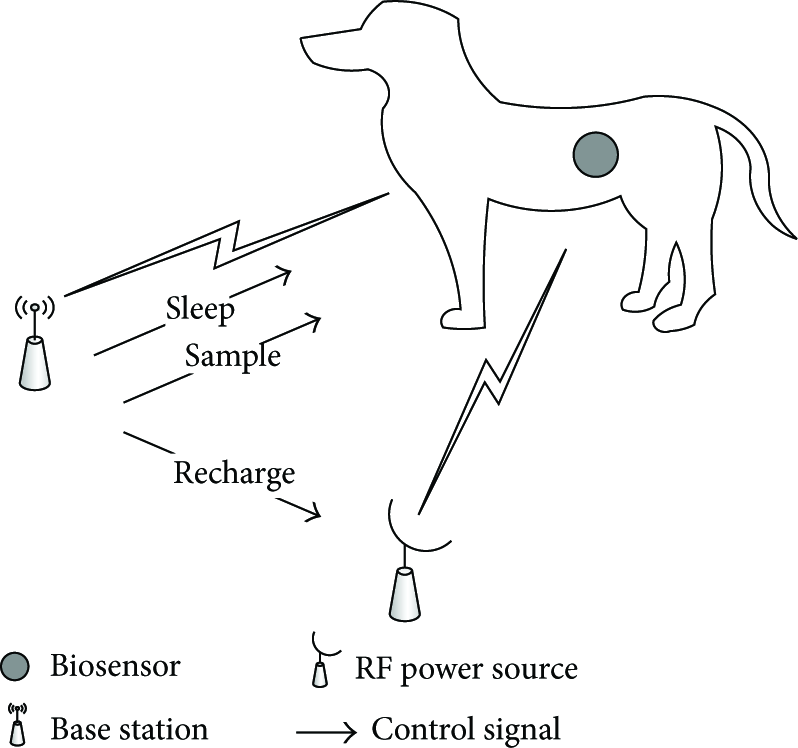
Setup of the system under study.

Both the biosensor and RF power source are under the control of the base station which initiates the measurement process. The base station generates three control signals: Sleep and Sample targeted at the biosensor and Recharge targeted at the RF power source. The system state information is assumed to be available to the base station before it generates a control signal.

Mathematically, the system can be modeled as a discrete-state system which evolves in discrete time. Therefore, the time axis is divided into slots of equal durations $\mathrm{\Delta }t$ . At the beginning of each time slot, the state of the system is observed and a control signal is generated by the base station accordingly. Each time slot is long enough to transmit a complete packet carrying a measurement. Next, the elements of the system are described.

4.1. Biosensor

A biosensor typically contains four essential components: biorecognition, transducer, radio and battery. The biorecognition system is made of elements such as enzymes and antibodies whose role is to produce a physio-chemical change which is detected and measured by the signal transducer. The transducer carries out signal processing tasks. The radio circuitry is responsible for wireless communication. The battery provides power for all active modules in the biosensor and is recharged using RF energy. During a recharging period, the biosensor uses its radio module to collect energy and recharge the battery. Therefore, while its battery is being recharged, the biosensor cannot perform sensing and communication.

The location of a biosensor represents a critical point since it experiences the maximum temperature increase. This is because the tissues surrounding the biosensor might be heated continuously due to the local radiation generated by the biosensor itself and the radiation generated by the base station while recharging the biosensor.

In each time slot t, the state of the biosensor is characterized by two variables which are the current temperature $T_t$ and energy level $E_t$ . There are $\tau +\mathrm{1}$ safe temperature levels; that is, $T_t\in \{\mathrm{0,1},\dots ,\tau \}$ , where the zero temperature level represents the normal body temperature and τ is an upper limit which must not be exceeded. Initially, the biosensor has a total energy of ${ℰ}_{\mathrm{0}}$ which is also the capacity of its battery. The energy required for the biosensor to successfully transmit its measurement to the base station is determined by the state of the wireless channel at the time of transmission. This transmission energy is denoted by ${ℰ}_{w_i}$ , where $w_i$ is the ith state of the wireless channel. The temperature increase due to a transmission energy of ${ℰ}_{w_i}$ units is denoted by ${𝒯}_{w_i}$ .

At the beginning of each time slot, the base station may decide to recharge the biosensor; let it transmit its measurement or put it into sleep. The time required for a full recharge is random since it depends on the current temperature and energy levels. During this time, interesting events may occur but they will not be reported by the biosensor since it is being recharged. Also, the biosensor may be put into sleep for a random amount of time during which no measurements can be produced.

At the beginning of the next time slot (i.e., $t+\mathrm{1}$ ), the energy level at the biosensor is given by the following equation:

$$\begin{array}{cc}& E_{t+\mathrm{1}}=\{\begin{array}{cc}{E}_t\hfill & \text{if}\hspace{0.17em}\hspace{0.17em}{a}_t=Sleep\hfill \\ E_t-{ℰ}_{w_i}\hfill & \text{if}\hspace{0.17em}\hspace{0.17em}{a}_t=Sample\hfill \\ E_t+{ℰ}_r\hfill & \text{if}\hspace{0.17em}\hspace{0.17em}{a}_t=Recharge,\hfill \end{array}\end{array}$$

(5)

where $a_t$ is the action taken by the base station at time t and ${ℰ}_r$ is the amount of energy gained by the biosensor. Similarly, the temperature of the biosensor at $t+\mathrm{1}$ is given by the following equation:

$$\begin{array}{cc}& T_{t+\mathrm{1}}=\{\begin{array}{cc}\max \{T_t-{𝒯}_s,\mathrm{0}\}\hfill & \text{if}\hspace{0.17em}\hspace{0.17em}{a}_t=Sleep\hfill \\ T_t+{𝒯}_{w_i}\hfill & \text{if}\hspace{0.17em}\hspace{0.17em}{a}_t=Sample\hfill \\ T_t+{𝒯}_r\hfill & \text{if}\hspace{0.17em}\hspace{0.17em}{a}_t=Recharge,\hfill \end{array}\end{array}$$

(6)

where ${𝒯}_s$ is the amount by which the temperature of the biosensor decreases when it is put to sleep. In the same way, ${𝒯}_r$ and ${𝒯}_w$ are the amounts by which the temperature of the biosensor increases when it is recharged and when it is allowed to transmit its measurement, respectively. ${𝒯}_r$ and ${𝒯}_w$ can be calculated using (4). ${𝒯}_r$ is constant since the SAR due to the base station is assumed to be constant. On the other hand, ${𝒯}_w$ is not constant since the SAR due to the biosensor changes with the change in transmission energy. Therefore, before ${𝒯}_w$ can be calculated, the SAR due to the radiation from the antenna of the biosensor is calculated using (2). Since (2) is a function of I, it is assumed that the current (I) corresponding to each transmission power level is known.

4.2. Wireless Channel

The communication between the biosensor and base station occurs over a Rayleigh fading channel with additive Gaussian noise. Hence, the instantaneous received Signal-to-Noise Ratio (SNR) denoted by γ is exponentially distributed with the following probability density function [12]:

$$\begin{array}{cc}& P\left(\gamma \right)=\frac{\mathrm{1}}{{\gamma }_{\mathrm{0}}}\exp \left(-\frac{\gamma }{{\gamma }_{\mathrm{0}}}\right),\end{array}$$

(7)

where ${\gamma }_{\mathrm{0}}$ is the average received SNR.

Such a wireless channel can be modeled as a Finite-State Markov Chain (FSMC) [13, 14]. The model can be built as follows. For a wireless channel with K states, the state boundaries (i.e, SNR thresholds) are denoted by ${\mathrm{\Gamma }}_{\mathrm{1}},{\mathrm{\Gamma }}_{\mathrm{2}},\dots ,{\mathrm{\Gamma }}_K,{\mathrm{\Gamma }}_{K+\mathrm{1}}$ , where ${\mathrm{\Gamma }}_{\mathrm{1}}=\mathrm{0}$ and ${\mathrm{\Gamma }}_{K+\mathrm{1}}=\infty$ . The channel is said to be in state $s_i$ if the SNR is between ${\mathrm{\Gamma }}_i$ and ${\mathrm{\Gamma }}_{i+\mathrm{1}}$ , where $i=\mathrm{1,2},\dots ,K$ . It is assumed that the SNR remains the same during packet transmission, and only transitions to the current or adjacent states are allowed.

The steady-state probability of the ith state of the FSMC is given by

$$\begin{array}{cc}& P\left(s_i\right)=\exp \left(-\frac{{\mathrm{\Gamma }}_i}{{\gamma }_{\mathrm{0}}}\right)-\exp \left(-\frac{{\mathrm{\Gamma }}_{i+\mathrm{1}}}{{\gamma }_{\mathrm{0}}}\right)\end{array}$$

(8)

and thus the state transition probabilities are

$$\begin{array}{cc}& P\left(s_{i+\mathrm{1}}\mid s_i\right)\approx \frac{N\left({\mathrm{\Gamma }}_{i+\mathrm{1}}\right)\mathrm{\Delta }t}{P\left(s_i\right)},\\ P\left(s_{i-\mathrm{1}}\mid s_i\right)\approx \frac{N\left({\mathrm{\Gamma }}_i\right)\mathrm{\Delta }t}{P\left(s_i\right)},\end{array}$$

(9)

where $N({\mathrm{\Gamma }}_i)$ is the average number of times per unit interval that the SNR crosses level ${\mathrm{\Gamma }}_i$ and $\mathrm{\Delta }t$ is the packet duration. $N({\mathrm{\Gamma }}_i)$ can be computed using the following equation [15]:

$$\begin{array}{cc}& N\left({\mathrm{\Gamma }}_i\right)=\sqrt{\mathrm{2}\pi {\mathrm{\Gamma }}_i}{f}_d{e}^{-{\mathrm{\Gamma }}_i},\end{array}$$

(10)

where $f_d$ is the maximum Doppler frequency defined as $f_d=v/\lambda$ with v being the speed of the subject and λ being the wavelength.

The above channel model has been verified to be precise when the fading process is slow [13], such as in biosensor applications.

5. MDP Formulation

An MDP is a model of a dynamic system whose behavior varies with time. The elements of an MDP model are the following [16]:

• (1)

system states,

(2)

possible actions at each system state,

(3)

a reward or cost associated with each possible state-action pair, and

(4)

next state transition probabilities for each possible state-action pair.

The solution of an MDP model (referred to as a policy) gives a rule for choosing an action at each possible system state. If the policy chooses an action at time t depending only on the state of the system at time t, it is referred to as a stationary policy. An optimal stationary policy exists over the class of all policies if every stationary policy gives rise to an irreducible Markov chain. This means that one can limit the attention to the class of stationary policies.

In order to obtain a policy from an MDP model, it is necessary to form and solve the so-called optimality equation (or Bellman's equation). The following is the standard form of this equation with the maximization operator [17]:

$$\begin{array}{cc}& V_n\left(s\right)=\underset{a\in A\left(s\right)}{\max }\left[\phantom{\sum _{s^{\prime }\in S}‍}f\left(s,a\right)+\sum _{s^{\prime }\in S}‍\mathbb{P}\left(s,s^{\prime },a\right)V_{n-\mathrm{1}}\left(s^{\prime }\right)\right],\end{array}$$

(11)

where n is the iteration index, S is the set of system states ( $s\in S$ ), $A(s)$ is the set of actions possible when the system is at state s, $f(s,a)$ is the reward/cost per step, ℙ is the system state transition probability matrix, and $V(s)$ is the optimal value of the objective function when the system is started at state s and the optimal policy is followed. Equation (11) can be solved using the classical policy iteration, value iteration, and relative value iteration algorithms [17]. Next, the details of the MDP model are given.

5.1. State Set

The state of the system at time t is described by the following 3-dimensional vector:

$$\begin{array}{cc}& s_t=(T_t,E_t,W_t),\end{array}$$

(12)

where $T_t$ , $E_t$ , and $W_t$ are the current temperature of the biosensor, its energy level, and transmission power required for successful transmission at time t, respectively. The total number of possible states is $|S|=|T|\times |E|\times |W|$ , where $|T|$ , $|E|$ , and $|W|$ are the numbers of possible temperatures, residual energies, and transmission energy levels, respectively.

5.2. Action Set

In each time slot, the base station chooses an action based on the current state of the system. In each state s, there are three possible actions:

$$\begin{array}{cc}& A\left(s\right)=\left\{Sample,Recharge,Sleep\right\},\end{array}$$

(13)

where the $Sample$ action lets the biosensor generate a measurement and transmit it to the base station, $Recharge$ action recharges the biosensor, and $Sleep$ action puts the biosensor into sleep.

The Sleep action can be performed at every system state. The other two actions, however, can only be performed at system states, where the next temperature of the biosensor is within the safe temperature range. In addition, the Sample action can only be performed at system states, where the remaining energy is sufficient to make a successful transmission.

5.3. Reward Function

Since the objective is to maximize the expected number of samples that can be generated by the biosensor, the reward function is defined as

$$\begin{array}{cc}& R(s,Sample)=\mathrm{1}.\end{array}$$

(14)

This means that one unit of reward is earned every time the Sample action is performed. The long-run expected sum of rewards represents the average number of samples that can be generated by the biosensor with an initial energy of ${ℰ}_{\mathrm{0}}$ units and maximum temperature increase of τ units.

5.4. Transition Probability Function

After the action taken by the base station is performed, the system transits to a new state according to the transition probabilities of the present state of the wireless channel. Thus, the behavior of the system is described by $|A|$ transition probability matrices, and each such matrix is of size $|S|\times |S|$ . Each matrix is denoted by $P_{s_t,s_{t+\mathrm{1}}}(a)$ which is the probability that choosing an action a when in state $s_t$ will lead to state $s_{t+\mathrm{1}}$ . More formally, $P_{s_t,s_{t+\mathrm{1}}}(a)$ can be written as follows:

$$\begin{array}{cc}& P\left[s_{t+\mathrm{1}}\mid s_t,a_t\right]=P\left[W_{t+\mathrm{1}}\mid W_t\right].\end{array}$$

(15)

5.5. Value Function

The problem of finding an optimal policy for maximizing the average number of samples is formulated as an infinite-horizon MDP using the average reward criterion [16]. So, let $V_{\pi }(s_{\mathrm{0}})$ be the expected number of samples given that the policy π is used with an initial state $s_{\mathrm{0}}$ . Then, the maximum expected number of samples $V^{*}(s_{\mathrm{0}})$ starting from state $s_{\mathrm{0}}$ is given by

$$\begin{array}{cc}& V^{*}\left(s_{\mathrm{0}}\right)=\underset{\pi }{\max }{V}_{\pi }\left(s_{\mathrm{0}}\right).\end{array}$$

(16)

The optimal policy ${\pi }^{*}$ is the one that achieves the maximum expected number of samples at all system states.

The famous value iteration algorithm [17] is used to numerically solve the following recursive equation for $n>\mathrm{0}$ :

$$\begin{array}{cc}& V_n\left(s\right)=\underset{a\in A\left(s\right)}{\max }\left[\phantom{\sum _{s_{t+\mathrm{1}}\in S}‍}R\left(s,a\right)+\sum _{s_{t+\mathrm{1}}\in S}‍\mathbb{P}\left(s_t,s_{t+\mathrm{1}},a\right)V_{n-\mathrm{1}}\left(s_{t+\mathrm{1}}\right)\right].\end{array}$$

(17)

In (17), the subscript n denotes the iteration index. As $n\to \infty$ , $V_n\to V^{*}$ .

6. Handling Large-Size MDP Models

The size of the proposed MDP model depends on the number of biosensor states which is a function of the number of possible temperature and energy levels. As the number of biosensor states increases, the process of computing the transition probability matrices for the system becomes very time consuming. Also, the value iteration algorithm used for solving the MDP model becomes impractical. This section presents two methods (namely, Q-learning and heuristics) for handling MDP models with a large number of states.

6.1. Q-Learning

Reinforcement Learning (RL) offers an alternative for obtaining the optimal policy at a significantly lower computational cost. Using a simulation model of the system under study, the decision maker in an MDP is viewed as a learning agent whose task is to learn the optimal action in each possible state of the system. As Figure 2 shows, the optimal policy is learned while the system is being driven (i.e., simulated) by the actions selected by the learning agent which stores the results of its actions in a knowledge base. The actions of the decision maker become better over time as new knowledge is obtained. Eventually, the RL algorithm converges to an optimal policy which can be used in the physical system.

Figure 2

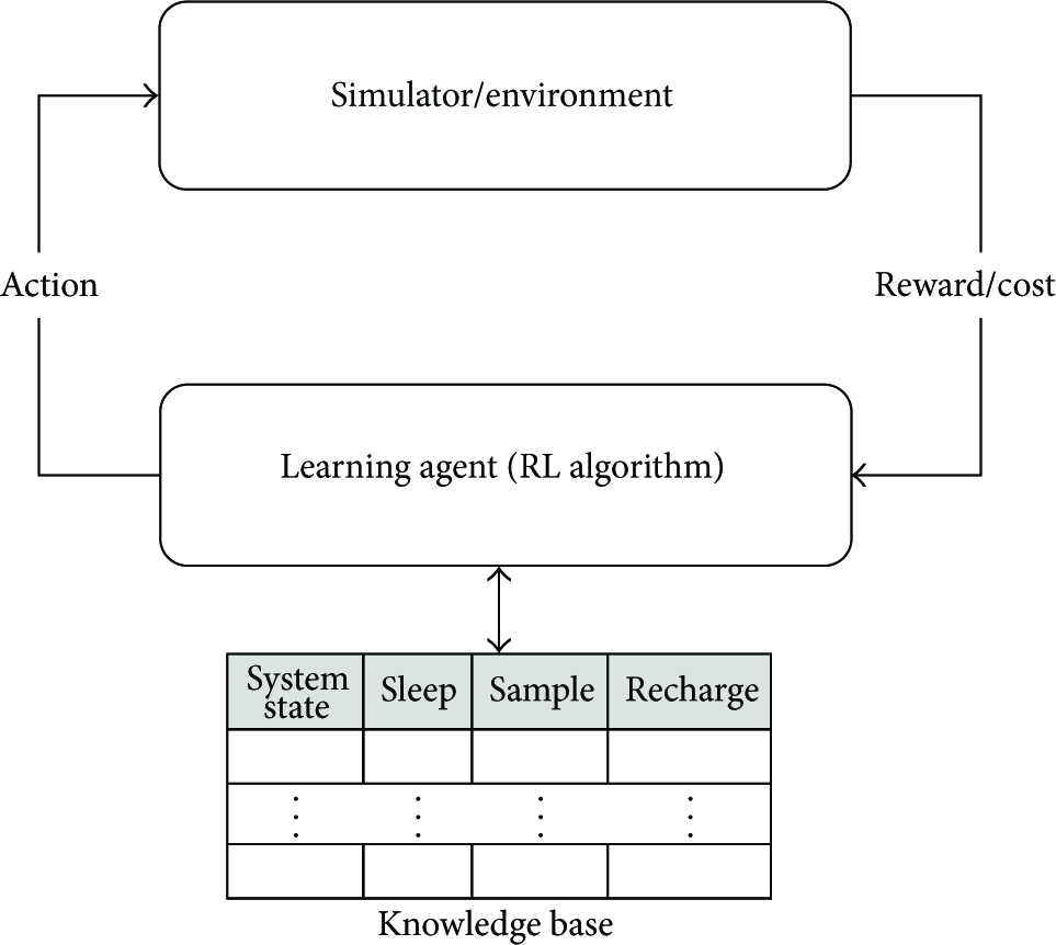
Using an RL algorithm (like Q-learning), the decision-making agent gradually learns the optimal policy. An action is applied to the system or simulated and then the resulting reward/cost is fed back into the knowledge base of the decision maker. The new knowledge obtained over time helps the decision maker to make better actions.

Q-Learning is an RL algorithm which was introduced in [18]. It is used for learning from experience. It requires that each entry in the decision-maker's knowledge base corresponds to a state-action pair. The value stored in each entry is referred to as the Q-value and is a measure of the goodness of executing an action in a particular system state. The Q-value for a state-action pair $(s,a)$ is updated as follows:

$$\begin{array}{l}Q\left(s,a\right)=Q(s,a)+\alpha \\ \hspace{1em}\hspace{1em}\hspace{1em}\hspace{1em}*\left(r+\gamma *\underset{j\in A\left(s^{\prime }\right)}{\max }Q\left(s^{\prime },j\right)-Q\left(s,a\right)\right),\end{array}$$

(18)

where r is the immediate reward obtained after executing action a in state s, $s^{\prime }$ is the next state, and $A(s^{\prime })$ is the set of possible actions in state $s^{\prime }$ . α and γ denote the learning rate and discount factor ( $\mathrm{0}<\gamma <\mathrm{1}$ ), respectively.

The Q-learning algorithm is shown as Algorithm 1. The interaction between the learning agent and the simulator (or environment) is divided into episodes. In each episode, the system transits through a sequence of states. The length of this sequence is controlled by the parameter $NumIter$ which is the number of simulated time slots. In each simulated time slot, based on the current state of the system, the learner chooses an action either based on the ϵ-policy or randomly. If the former is selected, the action with the highest Q-value is selected. After that, if the action is Sample, a reward of one unit is earned; otherwise, the reward is zero. The action is then simulated and the next system state is observed. Next, the Q-value is updated using (18). Also, the new system state becomes the current one and the cycle repeats.

Algorithm 1: The Q-Learning algorithm.

for   $i=\mathrm{1}$ to $NumEpisodes$   do

$\hspace{1em}ps\leftarrow InitialState$ ;  {E.g., [0 ${ℰ}_{\mathrm{0}}$ 1]}

 for   $j=\mathrm{1}$ to $NumIter$   do

  if   $rand\le \mathrm{1}-ϵ$   then

$\hspace{1em}\hspace{1em}\hspace{1em}a\leftarrow {\max }_{j\in \mathrm{\hspace{0.17em}\hspace{0.17em}}A(ps)}Q\left(ps,j\right)$ ;  {rand ∈ (0,1)}

  else

$\hspace{1em}\hspace{1em}\hspace{1em}a\leftarrow Random\hspace{0.17em}(A(ps))$ ;   {Random Action}

  end if

  if   $a==Sample$   then

$\hspace{1em}\hspace{1em}\hspace{1em}r\leftarrow \mathrm{1}$ ;  {Reward}

  else

$\hspace{1em}\hspace{1em}\hspace{1em}r\leftarrow \mathrm{0}$ ;

  end if

$\hspace{1em}\hspace{1em}ns\leftarrow SimulateAction(ps,a)$ ;

$\hspace{1em}\hspace{1em}Update\hspace{0.17em}(Q(ps,a))$ ;  {Using (18)}

   $ps=ns$

 end for

end for

Although Q-learning is theoretically guaranteed to obtain an optimal policy, it requires that each state-action pair be tried infinitely often in order to learn the optimal policy. The quality of the learned policy depends on how much time is spent in learning and if every state-action pair can be tried. On the other hand, depending on the application, a certain percental difference between the learned and optimal policies might be tolerated. This is because the system states differ in the likelihood of being visited. Thus, a default action (like Sleep) can be assigned to system states with a low likelihood of being visited.

6.2. Heuristic

Since it is difficult to describe the structure of the optimal policy, a heuristic policy is proposed in this section. The goal is to design a policy which mimics the behavior of the optimal policy as close as possible. However, before presenting such a policy, a greedy one is given to provide insight into the design of any heuristic policy.

The greedy policy is computed using Algorithm 2. The inputs to this algorithm are the set of possible system states and the set of feasible actions for each system state. The computed policy is greedy in the sense that for each system state, the feasibility of actions is checked in the following order: Sample, Recharge, and then Sleep. The first feasible action is associated with the corresponding system state.

Algorithm 2: Greedy policy.

       S: Set of possible systemstates

Require:  A: Set of possible actions at

      each system state

 for   $i=1$ to $\left|S\right|$   do

     if Action (i, Sample) is True then

       Policy(i) = Sample

      else if Action (i, Recharge) is True then

       Policy(i) = Recharge

     else

       Policy(i) = Sleep

     end if

 end for

As will be shown by simulations in the next section, the greedy policy is poor since it is based on a fixed order of actions. Therefore, Algorithm 2 needs to be extended to allow for a dynamic selection of actions. This objective is accomplished by introducing two control parameters: α and β. With these two control parameters, the Sample and Recharge actions are not selected in a specific order or whenever they are feasible. Algorithm 3 shows how the control parameters and new heuristic policy are computed.

Algorithm 3: Heuristic policy.

      S: Set of possible system states

Require:  A: Set of possible actions at

      each system state

$\hspace{1em}\alpha =T/\tau$

$\hspace{1em}\beta =E/E_0$

 for   $i=1$ to   $\left|S\right|$   do

  if Action (i, Sample) is True and $\alpha \le \beta$   then

     Policy (i) = Sample

  else if Action (i, Recharge) is True and $\alpha \ge \beta$   then

     Policy (i) = Recharge

  else

     Policy (i) = Sleep

  end if

 end for

The essence of Algorithm 3 is as follows. If the current temperature (denoted by T) of the biosensor is low and its current energy level (denoted by E) is high, then the condition $\alpha \le \beta$ would more likely be true and thus the Sample action could be executed. However, this would not be the case when the available energy is very close to zero. In this case, the opposite condition (i.e., $\alpha \ge \beta$ ) would more likely be true and thus a Recharge could be performed. If neither of the two conditions is true, the biosensor is put to sleep and thus its temperature decreases.

7. Numerical and Simulation Results

In this section, an example is first presented to illustrate the viability of the proposed MDP model. Then, the performance of the optimal policy is compared to that of the approximate policies using simulation. The impact of various system parameters on the performance of the system is also evaluated. The simulation was performed using a simulator written in Matlab [19]. Each simulation was run for a duration of 100000 time slots, and each data point is the average of 10 simulation runs. The number of channel states (W) is four, and the channel state boundaries are randomly generated.

7.1. Illustrative Example

In this example, a wireless channel with two states is considered. The channel state transition probabilities are calculated using (9). Table 1 shows the values of the parameters involved. Figures 3(a) and 3(b) show the expected number of samples when there is no recharge and when recharge is allowed, respectively. The expected number of samples is expressed as a function of the maximum safe temperature level (τ) and initial energy ( ${ℰ}_{\mathrm{0}}$ ). The first observation is that if recharge is allowed, more samples are expected to be generated by the biosensor. In the case when recharge is not allowed, the expected number of samples is limited only by the amount of initial energy. This is confirmed by Figure 3(a) where for the same initial energy, the same expected number of samples is obtained when τ is varied.

Table 1

Values assigned to the parameters of the example and Q-learning algorithm.

	Parameter	Value
Example	$\mathrm{\Delta }t$	0.25 ms
	$f_d$	60 Hz
	${ℰ}_{\mathrm{0}}$	5
	T	5
	${ℰ}_{w_{\mathrm{1}}}$ , ${ℰ}_{w_{\mathrm{2}}}$	1, 2
	${𝒯}_{w_{\mathrm{1}}}$ , ${𝒯}_{w_{\mathrm{2}}}$	1, 2
	${𝒯}_s$	1
	${𝒯}_r$	1
	${ℰ}_r$	1
Q-Learning	$NumEpisodes$	100
	$NumIter$	10000
	ϵ	0.5
	α	0.2
	γ	0.1

Figure 3

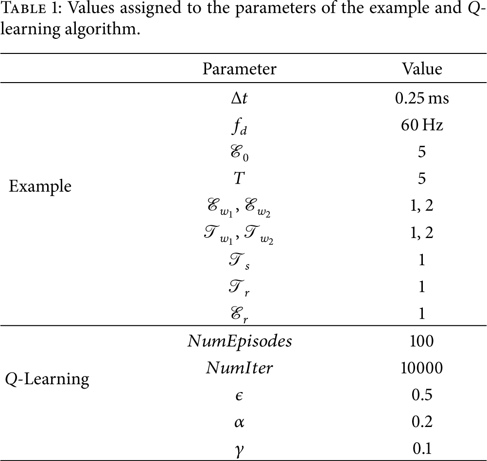
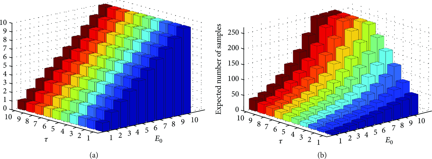
Expected number of samples. (a) No recharge. (b) With recharge.

When recharge is allowed, the maximum safe temperature level (τ) plays a critical role. This is due to the temperature increase caused by the recharge action. In Figure 3(b), for the same initial energy, the expected number of samples increases as τ is varied. Increasing τ enables the Recharge action to be performed more often. On the other hand, as one would expect, if τ is fixed and ( ${ℰ}_{\mathrm{0}}$ ) is varied, the expected number of samples slightly increases when τ is small. However, when τ is large (≥6), the maximum possible expected number of samples can be achieved when ${ℰ}_{\mathrm{0}}$ is at its maximum value. Therefore, for this particular example, if ${ℰ}_{\mathrm{0}}=\mathrm{10}$ , the optimal value for τ is 6.

Figures 4(a) and 4(b) show the optimal action for each possible system state. In Figure 4(a), for channel state 1, the Sample action is performed in $\mathrm{70}\%$ of the system states. The Sleep action is performed whenever the temperature reaches the maximum safe level (τ), and the Recharge action is performed when the remaining energy is zero and the temperature is below τ.

Figure 4

Optimal policy for τ = 5 and ${ℰ}_{\mathrm{0}}$ = 5. Actions 1, 2, and 3 denote Sample, Recharge, and Sleep, respectively. (a) Policy for channel state 1. (b) Policy for channel state 2.

By contrast, in Figure 4(b), for channel state 2, the Sample action is performed only once at the initial system state. For this channel state, due to the higher cost of transmission, the biosensor is put in the sleep mode most of the time. However, since the cost of the Recharge action is independent of the channel state, the system recharges itself more often to enable more samples to be generated when the wireless channel switches to a state with a lesser transmission energy requirement (i.e., channel state 1).

7.2. Comparative Analysis

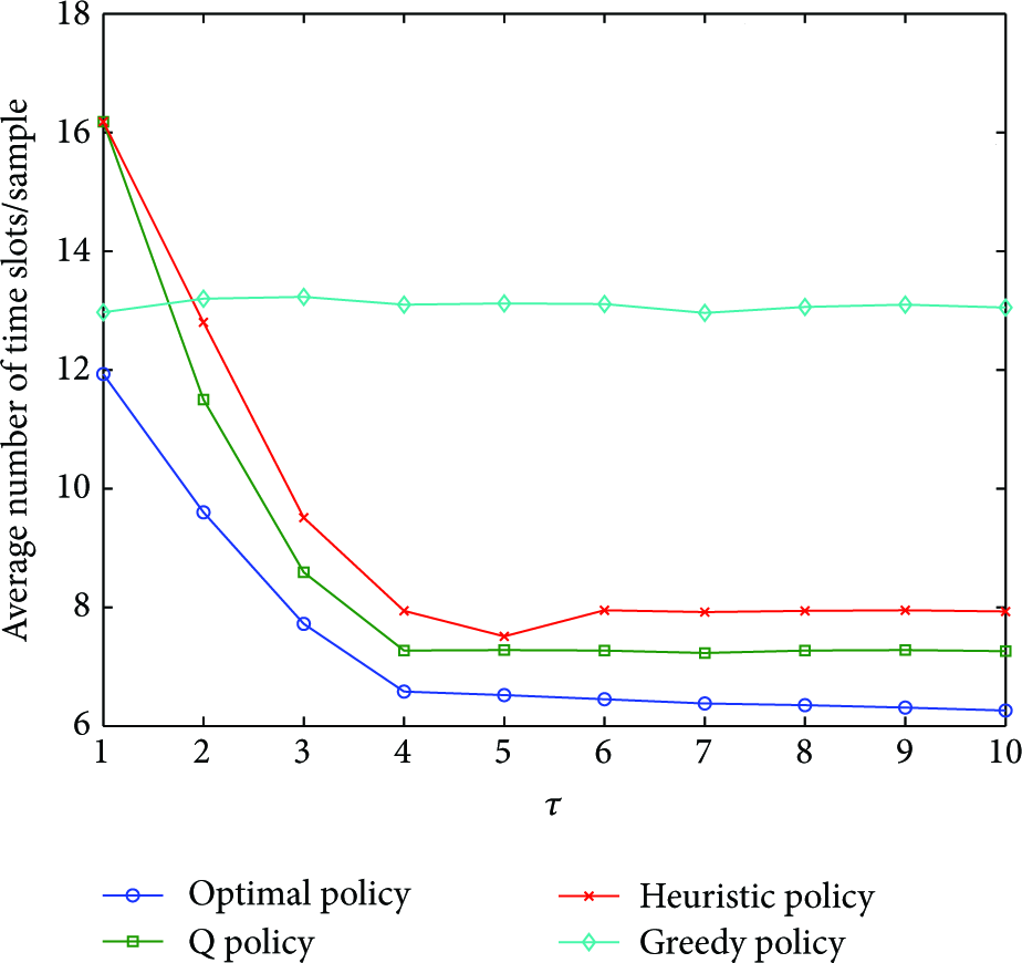
In order to be able to appreciate the merit of any approximate policy, a more meaningful performance criterion is needed. In this work, the average number of time slots needed to generate a sample is used as a criterion to distinguish between the different policies available to run a system. It is calculated as the total simulation time divided by the average number of samples generated by the system while being operated by a certain policy. This measure takes into account the effect of the Recharge and Sleep actions.

For example, consider Figure 5. In this figure, τ is fixed at five while ${ℰ}_{\mathrm{0}}$ is varied. The greedy policy is very costly since it requires the largest amount of time before a sample can be generated. The difference in the amount of time required by the heuristic policy and that required by the optimal policy stays around two time slots. This is a 75% reduction in time when compared to the greedy policy. The Q policy is the best approximate policy. On average, the difference with the optimal policy stays around 1.1 time slots.

Figure 5

Average number of time slots needed to generate a sample when τ is fixed at five and ${ℰ}_{\mathrm{0}}$ is varied.

Figure 6 shows the amount of time required to generate a sample when ${ℰ}_{\mathrm{0}}$ is fixed at five and τ is varied. In this figure, when $\tau =\mathrm{1}$ , the greedy policy outperforms both the Q policy and heuristic policy. A difference of three time slots is observed. This can be explained as follows. In the Q and heuristic policies, the Recharge action can be performed in one state only (i.e., when $T=E=\mathrm{0}$ ). On the other hand, with the greedy policy, the Recharge action can be performed in more than one state (i.e., whenever $T=\mathrm{0}$ ). This, of course, leads to a reduction in the average amount of time needed to generate a sample. Other than that, for $\tau \ge \mathrm{2}$ , the Q and heuristic policies are always better than the greedy policy, and their performance is close to that of the optimal policy.

Figure 6

Average number of time slots needed to generate a sample when ${ℰ}_{\mathrm{0}}$ is fixed at five and τ is varied.

8. Conclusions

The increase in temperature due to the heat generated by biosensors is a limiting factor in the operation of biosensor networks. This problem can be modeled as a stochastic control problem using the framework of Markov decision processes. The solution is an optimal policy which ensures that the maximum safe temperature level is not exceeded. In order to handle large-size MDP models, it is shown how Q-learning can be used for obtaining the optimal policy. In addition, a heuristic policy is proposed. Its performance is comparable to that of the policies obtained by the MDP model and Q-learning.

This work can be extended in the following directions. First, the scenario of more than one rechargeable biosensor should be studied. In this case, the number of possible system states is exponentially huge. Thus, techniques for eliminating equivalent states would be necessary. Second, the performance of other reinforcement learning techniques should be investigated, especially for models with a huge state space. Third, algorithms for computing better heuristic policies should be developed to mitigate the problem of finding better approximate policies.