Sage Journals: Discover world-class research

Abstract

A high-resolution vision system for the inspection of drilling tools is presented. A triangulation-based laser scanner is used to extract a three-dimensional model of the target aimed to the fast detection and characterization of surface defects. The use of two orthogonal calibrated handlings allows the achievement of precisions of the order of few microns in the whole testing volume and the prevention of self-occlusions induced on the undercut surfaces of the tool. Point cloud registration is also derived analytically to increase to strength of the measurement scheme, whereas proper filters are used to delete samples whose quality is below a reference threshold. Experimental tests are performed on calibrated spheres and different-sized tools, proving the capability of the presented setup to entirely reconstruct complex targets with maximum absolute errors between the estimated distances and the corresponding nominal values below 12 μm.

1. Introduction

In the last few decades, starting from the early 1950's, the coordinate measurement machines (CMMs) have gained increasing importance in quality control in manufacturing industries up to play a key role in the inspection of complex assemblies in many mechanical fields, such as aeronautics and automotive.

Conventional CMMs can be represented as made of three simple blocks: a handling system for three-dimensional (3D) motion, a touching probe, and a data collector. Although many techniques aimed to reduce measurement uncertainty had been proposed [1 –3], touching probes are implicitly sources of limitations in their applications. For instance, these systems can be unsuitable for delicate objects that could be damaged by an improper pressure or can lead to ambiguous measurements when the probe itself is deflected by the target.

For these reasons, contactless optical probes have been developed in order to get reliable measurements when the drawbacks of contact systems limit their effective applicability [4, 5]. Among them, those based on laser triangulation are very promising since they are not invasive and provide high precisions and fast measurements, whereas the low optical crosstalk and the high contrast gained by the use of laser sources allow the suppression of the noise level [6 –11]. Additionally, the high accuracy attainable exploiting laser scanning systems have opened the way for many new applications in different fields beyond mechanics, such as reverse engineering [12, 13], plastic surgery [14, 15], environmental reconstruction [16], and cultural heritage [17, 18]. Typical pros and cons of 3D optical sensors in relationship with the application fields have been clearly presented and discussed in [19].

The design of a laser triangulation scanner presents many challenges mainly ascribable to the accurate calibration of the whole system, the extraction of laser spots displayed on the camera plane, the presence of second-order reflections superposed on the actual meaningful signal, and the speckle noise sources [20, 21]. Many works have been done by researchers in order to achieve error compensation [22, 23] and the deep understanding of how the choice of the setup parameters can alter the results of the measurements [24]. Moreover, the inspection of complex surfaces can lead to self-occlusions when the field of view of the optical probe is cloaked by more external regions of the object under investigation. The first idea to solve this problem regards the use of path-planning techniques [25 –27]. This issue is intended to find the best path, in terms of subsequent viewpoints for each laser scanning, that allows the complete coverage of the testing target, meeting some quality criteria on the reconstructed point cloud. This means that when the CAD model of the object is given, critical points are determined and a scanning path is then generated by checking the superimposed criteria. On the contrary, when CAD models of the target are not available, predictive blocks are integrated in the control system to define the following motion trajectories of the optical probe.

All the presented techniques have an important drawback that resides in the time required to perform a single acquisition, due to the need of preprocessing data to control the quality of results. In this paper, a high-resolution triangulation-based laser scanner is presented for the 3D reconstruction of complex objects. The field of application of the proposed system regards the entire characterization of drilling tools, whose geometry makes challenging their analysis. In particular, the presence of sharp edges, undercut surfaces, and fast repetitions of concave and convex regions induces occlusions together with the reduction of the quality of the measurement. As a consequence, these aspects have to be compensated through the use of suitable techniques. First, a procedure able to solve occlusion problems by handling the optical probe is presented together with the development of a robust analytical method for the exact data registration. Then, a filtering technique for image processing is defined to reduce the negative effects due to light scattering and second-order reflections. A calibration procedure is finally derived for the setting-up of a measurement prototype. The validation of the system is obtained through the analysis of a calibration sphere, with results in good agreement with the expected ones (absolute error in radius computation of few microns). Further experiments prove the capability of the prototype to investigate the shape of different-sized tools with the aim of looking for surface defects.

This paper is organized as follows: in Section 2, the analytical framework is introduced for the analysis of simple nonoccluded targets and then extended to more complex cases with undercut regions; the prototype description and the implemented image processing are reported in Section 3, whereas the calibration pipeline and the setup validation are highlighted in Section 4; Section 5 shows experimental results of measurements on macro- and microtools, while final conclusions and remarks are in Section 6.

2. Analytical Framework

As shown in the previous section, the problem of laser triangulation had been widely discussed by researchers and its solution had been used in many industrial applications. In the following subsections, the acquisition strategy will be described under two different conditions. In the first case, the tool does not present self-occlusions due to undercut surfaces. Then, this condition is removed giving rise to an exhaustive analytical formulation of the problem. Further analyses are provided in order to define a strategy able to prevent the resolution decreasing due to the finite depth-of-field (DOF) of the elements of the setup.

2.1. Simple Case without Self-Occlusions

In two dimensions, the problem of laser triangulation can be addressed as shown in Figure 1 (a). A laser beam impinging on a target surface is revealed on the sensor plane of a camera. The set is made by the laser source and the camera constitutes the optical probe of the system.

Figure 1:

Sketches for the description of the principles of laser triangulation: (a) normal translation of a target surface and (b) simplified view of the presented system highlighting the adopted reference of coordinates.

As known, a rigid translation d of the surface along the direction parallel to the optical axis of the laser is translated in a shift Δp of the reveled laser spot on the camera plane. For convenience, we assume that the camera is oriented in order that the pixel displacement is displayed vertically; that is, Δp is a difference of row coordinates in the camera plane. This relationship between d and Δp can be easily expressed by the following:

d = k \frac{Δ p}{\sin α},

(1)

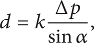
where α is the triangulation angle in Figure 1 (a), whereas k is a term which reports the camera coordinates in the metric reference system. This term is implicitly related to the camera lenses and to the physical dimensions of the pixels of the camera. Since traditional lenses induce optical distortions, k nonlinearly depends on the position of the revealed spot within the camera plane. In order to avoid the nonlinear behavior of the term k, a telecentric lens can be adopted, thus giving

k = \frac{s_{p}}{M},

(2)

with s_p being asthe size of the camera pixel and M as the magnification of the telecentric lens. It is important to remark that the constant term s_p/(Msinα) represents the conversion factor from the vertical pixel coordinate on the camera plane to the metric one along the direction of d.

All the considerations reported before are valid for a single dot impinging the target surface, accordingly to the two-dimensional definition of the problem. This framework can be exported in 3D by considering an extended laser line. In this case, the laser line can be treated as an array of laser spots, whose horizontal positions give information about the displacement d in the third direction. Analytically, the third component can be easily translated in metric coordinates by multiplying the column coordinate of the corresponding pixel by the term k in (2).

Since this work is devoted to the efficient reconstruction of drilling tools, the actual setup can be drawn as in Figure 1 (b) where a top view of the system is returned. In this case, the scanning of the tool is obtained by rotating the target around its drill axis, sampling the θ-axis with N_A points between 0 and 2π. Each frame captured by the camera reports the laser line distorted by the tool surface for a particular discrete angle θ_i, i = 1, …, N_A. This means that the term d in (1) has to be further transformed in order to get the actual coordinates of the corresponding point.

Under the hypothesis of infinite DOF of both laser and camera, and supposing that the field-of-view (FOV) of the camera is able to cover the whole volume of the tool, the generic ith laser line, acquired when θ = θ_i, spans horizontally the camera plane (see Figure 2), whose dimension is equal to N_C × N_R pixels. Line peaks can be detected at coordinates $(I_{j}^{(i)}, J_{j}^{(i)})$ , where j = 1, …, N_C, which correspond the 3D real coordinates $(X_{j}^{(i)}, Y_{j}^{(i)}, Z_{j}^{(i)})$ expressed as follows:

\begin{matrix} X_{j}^{(i)} = \frac{s_{p}}{M \sin α} (J_{0} - J_{j}^{(i)}) \cos θ_{i}, \\ Y_{j}^{(i)} = \frac{s_{p}}{M \sin α} (J_{0} - J_{j}^{(i)}) \sin θ_{i}, \\ Z_{j}^{(i)} = - \frac{s_{p}}{M} I_{j}^{(i)} . \end{matrix}

(3)

Figure 2:

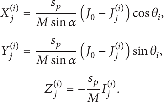
Schematic representation of the laser line reported on the camera plane.

It is worth noting that the pixel increment has to be related to a reference axis. All pixel measurements are computed as the gap between the actual row position of the line peak and the drill axis reported on the camera plane. Its location is independent of θ and always equal to J₀ for each column of the plane, since the drill axis is aligned to the z-axis, orthogonal to the xy-plane. Moreover, the sign of $Z_{j}^{(i)}$ is added in order to get a consistent reference system, as the one reported in Figure 1 (b).

Once the real coordinates of each detected point are determined, measurement resolutions can be derived. For convenience, these terms can be expressed in cylindrical coordinates (r, θ, z):

\begin{matrix} d r = \frac{s_{p}}{M \sin α}, \\ d θ = θ_{i + 1} - θ_{i}, \\ d z = \frac{s_{p}}{M} . \end{matrix}

(4)

All resolution terms related to distance measurements are directly influenced by s_p and M, whose ratios have to be as small as possible, within the limits imposed by the camera fabrication technologies. Quantitatively, this ratio sets dz equal to 2.2 μm. At the same time, the triangulation angle α participates in the expression of the resolution terms dr, in the sense that its sine function has to be kept as high as possible to get lower values of dr. This means that the closer to π/2 this angle is, the better radial resolution is reached. However, this condition is not realistic since high values of α induce occlusions while scanning the tool surface. A good balance can be struck by considering α close to π/4, which leads to dr equal to about 3.1 μm. Finally, the angular resolution dθ directly depends on the angular aperture between two successive frames acquired by the camera, that is, on the value assumed by N_A. Under the assumption that the rate of change of the angular displacement can be arbitrarily adjusted, this term is only limited by the initial specification regarding the time required for the entire reading of the tool, in relationship to the camera frame rate. The experimental settings adopted in this paper bring to an angular resolution of 0.7° at a camera frame rate of 25 fps.

2.2. Complex Case with Self-Occlusions

The visual inspection of drilling tools is challenging because of the presence of undercut regions that induce self-occlusions of several articulated surfaces. In many cases, the reconstruction of these surfaces is mandatory for the complete quality control of the tool. The problem of self-occlusions is shown in Figure 3, where undercut regions of the tool are reported in green.

Figure 3:

Acquisition schemes for the reconstruction of the whole surface of a complex tool. (a) Simple acquisition with θ_i = 0; (b) first scanning round with increasing θ_i for the evaluation of nonoccluded surfaces (blue edges); and (c) second scanning round with superimposed transversal shift t for the achievement of occluded surfaces (green edges).

By the analysis of Figures 3 (a) and 3 (b), it is clear that the single rotation of the tool around its axis is not able to reconstruct the surfaces of those undercut regions that are never reached by the laser line. This problem can be overcome by means of a transversal shift t of the optical probe. By this way, the laser line strikes the occluded surfaces at different rotation angles, whose value depends on the depth itself of the target surfaces. Moreover, the computed depth is also scaled by a factor still depending on the introduced shift t. Consequently, the process of point cloud registration is not merely subjected to a rotation of samples but is more complex and has to be computed analytically, knowing the term t.

With reference to Figure 4, where the two-dimensional problem is illustrated, the registration process aims to find the coordinates of the actual point P, corresponding to the point P′, illuminated under the conditions of a transversal shift t. Triangulation rules permit the definition of the distance $d_{j}^{(i, t)}$ from y-axis, starting from the knowledge of the jth pixel coordinates $(I_{j}^{(i, t)}, J_{j}^{(i, t)})$ of the detected laser line:

d_{j}^{(i, t)} = \frac{s_{p}}{M \sin α} (J_{0} - J_{j}^{(i, t)}) .

(5)

Figure 4:

Schematic view of a tool section (blue contours) for the analytical registration of occluded points acquired by imposing a transversal shift t of the optical probe. World coordinates (x, y) are used in this context.

The angle $γ_{j}^{(i, t)}$ is easily derived as

γ_{j}^{(i, t)} = ta n^{- 1} (\frac{t}{d_{j}^{(i, t)}}) .

(6)

Consequently, the radial component r_P′ of the point P′ can be written as

r_{P^{'}} = r_{P} = \frac{d_{j}^{(i, t)}}{\cos (γ_{j}^{(i, t)})} .

(7)

Once the radial component of the point P is identified, the actual coordinates of P can be obtained as the projection of r_P on the x- and y-axis, mediated by the angle $φ_{j}^{(i, t)}$ . In a more explicit way, the final 3D coordinates of the registered point P are

\begin{matrix} X_{j}^{(i, t)} = \frac{d_{j}^{(i, t)}}{\cos (γ_{j}^{(i, t)})} \cos (θ_{i} - γ_{j}^{(i, t)}), \\ Y_{j}^{(i, t)} = \frac{d_{j}^{(i, t)}}{\cos (γ_{j}^{(i, t)})} \sin (θ_{i} - γ_{j}^{(i, t)}), \\ Z_{j}^{(i, t)} = - \frac{s_{p}}{M} I_{j}^{(i, t)} . \end{matrix}

(8)

Finally, it is easy to verify that the formulations in (8) converge to those in (3) when the transversal shift vanishes.

It is worth noting that the choice of the term t is directly related to the shape and the size of the tool under analysis. In principles, only two values of t, roughly t₀ equal to 0 and t₁ smaller than the tool radius, are enough to overcome self-occlusions. Nevertheless, if surface holes still affect the resulting point cloud, more observations of the object have to be performed at intermediate values of t in the range [t₀, t₁].

2.3. Systems with Finite DOF

The formulations in (8) have been obtained under the fundamental hypothesis of infinite DOF of the element of the optical probe, both laser and camera, and considering a camera FOV able to cover the whole testing volume. In a more realistic scenario, these aspects are no longer valid. By looking at Figure 5 (a), it is evident how laser and camera DOFs, together with the Camera FOV, shrink the volume in which nominal resolutions are those in (4). This has effects on the downsizing of the exploitable area of the camera plane where the target is correctly focused. In fact, the decrease of the allowed depth, where (8) can be correctly estimated, leads to a consistent reduction of the region-of-interest (ROI) along the J-direction of the camera plane.

Figure 5:

Strategy for the preservation of the system resolution: (a) acquisition of external surfaces and (b) inspection of internal surfaces subsequent to the longitudinal shift l of the optical probe.

Preventing the measurement resolution from getting worse is mandatory in high-definition systems. This aim can be reached by adding a new degree of freedom to the optical probe, that is, a longitudinal shift l in the x-direction, which enables the acquisition of those internal surfaces that, otherwise, would not be captured. Each round of the tool at a particular l value defines an isodepth observation. All frames in a single round are thus labeled by the specific longitudinal shift l that is then used to reconstruct the coordinates of the reconstructed points. The expression of $d_{j}^{(i, t)}$ in (5) can be now rewritten as

d_{j}^{(i, t, l)} = \frac{s_{p}}{M \sin α} (J_{0} - J_{j}^{(i, t, l)}) + (l - l_{0}),

(9)

where l₀ represents the longitudinal shift needed to include the drill axis in the downsized ROI of the camera. The importance of this term will be further discussed in the Section 4 where the description of the calibration phase will be introduced.

The value of the parameter l has to be returned by an encoder able to transduce numerically the entity of the motion. These values are thus biased by an internal offset induced by the system of reference of the mechanical controller. Anyway, all values of l undergo the same offset that is then implicitly compensated by the term l₀.

3. System Prototype

Once the analytical formulations have been derived, the next step in the system design is the appropriate choice of the optical components. The next subsections will be devoted to the description of the prototype, together with a brief introduction on the steps followed for the image processing.

3.1. Experimental Setup

As underlined in the previous section, the optical probe is made of two main elements: the laser source and the optical receiver (camera and telecentric lens).

The properties of the laser source are the basis of the whole resolution of the proposed system, since, as expressed in (4), the capability of the algorithm of image processing to distinguish between two adjacent peak positions comes in succession to the quality of the laser line itself. In particular, the small thickness of the laser line over its entire length is a fundamental requirement to attain high resolutions. This goal can be achieved by means of a telecentric laser which produces a uniform lengthwise and Gaussian widthwise beam. Such specifications are guaranteed by a Lasiris TMFL-55 laser emitter, whose generated line thickness is equal to 9 μm (1/e² estimation) at its working distance. The main features of this device are reported in Table 1 [28].

Table 1:

Technical data of the Lasiris TMFL laser.

Parameter name	Parameter value

Depth of field	200 μm
Working distance	55 mm
Line width	9 μm
Line length	10 mm
Laser wavelength	660 nm
Output diode power	100 mW

The system resolution is also affected by the physical properties of the set made by the camera and the telecentric lens, which determines the ratio $s_{p} / M$ in (4). This ratio has to be set as low as possible in order to get the best conditions for the measurement resolution. Moreover, its value influences the sampling of the laser line that should lie widthwise over more than three pixels in order to enable efficient peak extraction strategies. The optical receiver is made of an IDS-uEye camera (Model USB-3-UI-3480CP-M) assisted by the telecentric lens Lensation TC5M-10-110i. The principal features of the lens and the camera are reported in Tables 2 and 3, respectively [30, 31].

Table 2:

Technical data of telecentric lens Lensation TC5M-10-110i.

Parameter name	Parameter value

Magnification	1X
Aperture (F)	6.5
Working distance	110 mm
Depth of field	260 μm

Table 3:

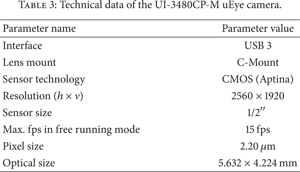
Technical data of the UI-3480CP-M uEye camera.

Parameter name	Parameter value

Interface	USB 3
Lens mount	C-Mount
Sensor technology	CMOS (Aptina)
Resolution (h × v)	2560 × 1920
Sensor size	1/2′′
Max. fps in free running mode	15 fps
Pixel size	2.20 μm
Optical size	5.632 × 4.224 mm

The proposed choice has results in a ratio $s_{p} / M$ equal to 2.2 μm. This value has to be further multiplied by the sine of the triangulation angle α in order to get the conversion factor from pixel shifts to metric displacements. Since typical values of α are close to π/4, the conversion term is approximately equal to 3 μm. This means that any laser line detected on the camera plane can be sampled in at least three pixels, as required.

Finally, it is important to observe that the laser source shows the minimum DOF of the elements of the optical probe (200 μm). As already discussed in Section 2.3, this value draws a line at the effective ROI within the camera plane, whose height has to be consequently reduced to approximately 70 pixels.

A picture of the prototype is highlighted in Figure 6, where the presence of micrometric slits which are only exploited during the calibration phase for the proper alignment of the optical components is evident.

Figure 6:

Picture of the prototype of the proposed setup. Micrometric slits are only used for the calibration phase of the acquisition process. All handlings, both translational and rotational, are numerically managed via an external controller. Legends describe corresponding setup components.

3.2. Image Processing

As shown previously, resolution can be further improved via image processing aimed to the detection of laser peaks with subpixel precisions. Starting from a single frame acquired by the camera, the laser line is scanned along the columns. Then, a couple of vectors including the row positions and the corresponding intensities of the illuminated pixels is extracted for each column containing the line. These two vectors are inputs for the detector, whose task is the estimation of the exact row position of the maximum laser intensity.

Many algorithms have been developed to determine the exact position of the laser peaks. Among these, the Gaussian approximation, linear interpolation, Blais and Rioux detectors, and parabolic estimators can be identified, just to mention a few [32].

Exploiting the knowledge of the physical shape of the emitted laser line, the implemented algorithm names the peak position as the expected value of the Gaussian distribution that fits the laser profile in the least squares sense. This method gives back an implicit quality index, that is, the standard deviation σ of the reconstructed Gaussian distributions. A simple threshold on this value is able to delete those peak estimations whose associate widths are higher than the expected ones (the threshold value σ_th), close to the nominal laser linewidth. Therefore, ambiguous estimations are removed preventing the increase of the measurement uncertainty. Henceforth, the mean value σ_av assumed by the standard deviations of the fitting Gaussian distributions will be used to express the quality of the reconstructed points.

Moreover, another threshold scheme can be used for the deletion of noise sources due to the presence of second-order reflections of light. Since noise signals have presumably lower light intensities, the peak extraction is enabled only when at least one pixel of the input vector has intensity higher than the threshold I_th. Therefore, columns that do not meet this specification are removed from the analysis, thus reducing also the computation time required for the image processing. This term has to be set properly depending on the emitted optical power. Experiments have proven that fixing I_th equal to a fraction of about 10–15% of the maximum laser intensity detected by the camera is enough to achieve the correct suppression of second-order reflections.

Further explication of how these terms affect results will be provided in the next paragraphs.

4. Preliminary Analysis

The preliminary phase of calibration of the setup is of primary importance for preventing systematic errors in the evaluation of relative distances among surfaces. In the following subsections, the calibration pipeline will be summarized together with the analysis of preliminary results of measurements carried out on a known target.

4.1. Calibration Pipeline

As can be seen in Figure 6, all optical components lie on positioning stages which introduce controlled translational shifts able to move separately the elements of the optical probe along the directions of the x-axis and y-axis. At the same time, two goniometers allow the rotations of both laser and camera around axes parallel to the corresponding optical directions.

The initial calibration phase can be listed as follows. Before starting, it is mandatory to notice that the calibration is run by placing a perfectly cylindrical tool with smooth surfaces in the mechanical spindle. Here, the radius of the tool is named r_c.

4.1.1. Positioning of Laser and Camera

The first step consists in checking the camera orientation. In this case, the laser is kept off and the camera is adjusted in order to focus on the cylindrical tool. The exposure time is then set high enough to get the tool smooth edge. The camera is thus oriented till the tool edge is perfectly aligned with the I-axis in Figure 2.

Then, the laser is fed with a suitable injection current and thus generates a line which impinges on the tool surface in the camera FOV. Hence, the laser source can be oriented till the produced line is perfectly aligned parallel to the I-axis of the camera plane.

Once both laser and camera are perfectly oriented, it is necessary to align the laser line on the drill axis. The laser source is shifted along the y-axis till the revealed line on the camera plane reaches the highest position along the J-axis. This position corresponds to the maximum distance from the drill axis; that is, the tool radius overlaps the x-axis.

Finally, laser and camera can be focused on the volume. This condition is found simultaneously by looking at the width of the detected laser line. The focus is reached when the laser linewidth reaches its minimum. Moreover, the focus coordinate along the J-axis of the camera plane determines the exact position of the ROI within the camera plane.

4.1.2. Choice of the Injection Current of the Laser

Scattering, specular reflections, and second-order reflections can worsen the measurement by increasing the width of the detected beam, although the laser line is correctly focused on the target surface. These aspects can limit the resolution of the system increasing the term dr over its nominal expected value.

Two different ways can be found to overcome this problem. The former is the fine-tuning of the feeding current of the laser in order to reduce its output power, thus finding the best condition against light scattering from the tool surface at the expense of the signal-to-noise ratio. The latter envisages modulation schemes of the laser amplitude. In this case, the camera has to be synchronized to the laser modulating signal in order to grab the line when the laser is switching off. For the sake of simplicity, the proposed setup exploits the first technique to preclude the deterioration of the line quality.

At this step, the cylindrical smooth tool is changed by a complex one, whose surface is made of rough edges. Its volume is coarsely scanned by the optical probe with different injection currents till the best balancing between the laser linewidth and the signal-to-noise ratio is reached.

4.1.3. Estimation of the Triangulation Angle

The correct estimation of the triangulation angle α is fundamental in the correct reconstruction of 3D points, since it affects the in-plane components $X_{j}^{(i, t, l)}$ and $Y_{j}^{(i, t, l)}$ , coming out form the peak coordinate $J_{j}^{(i, t, l)}$ .

This value can be obtained exploiting an inverse fit on the parameters in (1) and (2). In this case, the optical probe approaches and leaves the target surface of known quantities returned by the mechanical encoder. When the detected line falls in the camera ROI, the mean position of the extracted peaks along the J-axis can be recorded. The collection of data is used to solve an overdetermined system of linear equations as a function of α in the least squares sense. Figure 7 shows an example of data fitting where red dots are related to the experimental measurements, whereas the blue line is derived by the solution of the calibration problem.

Figure 7:

Results for the evaluation of the triangulation angle α. Experimental data (red dots) are obtained by moving the optical probe away from the target and recording the row coordinates of the detected laser lines. The blue line is the result of the curve fitting on the experimental data (depending on α).

4.1.4. Identification of the Position of the Drill Axis

As shown in the analytical formulation of the problem, each range measurement has to be referred to the drill axis, which is also the origin of the x-axis and y-axis. This contribution is carried by the terms l₀ and J₀ in (9). Explicitly, the aim of this preliminary phase is the determination of the value assumed by $((s_{p} / (M \sin α)) J_{0} - l_{0})$ , exploiting the simple technique reported in Figure 8.

Figure 8:

Scheme for the detection of the rotation axis of the tool. (a) Generic acquisition at the absolute encoder position E_x; (b) tuned acquisition run moving away the optical probe until the laser line lies on the boundary of the ROI on the camera plane (absolute encoder position E_x0). Windows show the snapshots of the ROI within the camera and the corresponding magnified views.

With reference to Figure 8 (a), as a first step, the optical probe is dragged playing on the x-handling to inspect the surface of the cylindrical tool. As a consequence, the laser line lies horizontally in the middle of the ROI, here 200-pixel-height, while the mechanical encoder returns an absolute position E_x. The optical probe is then moved away from the surface as far as the line reaches the edge of the ROI (Figure 8 (b)). Under this condition, the value E_x0 returned by the encoder is the actual distance of the ending depth boundary of the testing volume from the reference surface of the tool. Consequently, the exact position of the drill axis referred to the encoder system of coordinates can be derived by adding the known radius r_c of the cylindrical tool. This means that the objective term in (9) can be substituted by the sum (E_x0 + r_c), thus obtaining the following final formulation:

d_{j}^{(i, t, l)} = \frac{s_{p}}{M \sin α} (h_{ROI} - J_{j}^{(i, t, l)}) + (E_{x 0} + r_{c}) - l,

(10)

where l is now directly the shift value returned by the encoder, whereas h_ROI is the height of the ROI in the camera plane. It is important to underline that the condition presented in Figure 8 (b) has effects on the term J₀ in (9), now equal to h_ROI, as the laser line lies on the bottom of the camera ROI. Moreover, since the x-axis has origin in the center of the tool and comes out from it, in opposition to the handling system of reference, the term (l – l₀) has to change in sign in (9), thus converging to the formulation in (10).

4.2. Setup Validation

Before going through the analysis of experimental results, the calibrated system has to be validated with the inspection of a known target. In this case, a standard ceramic probe sphere with diameter equal to 18 mm is used. The robustness of this experimental validation is further guaranteed by the proper location of the calibration sphere. In particular, the alignment of the center of the sphere along the rotation axis is mediated by a high-precision mechanical comparator with results in a maximum positioning error of 2 μm. The results of laser scanning are reported in Figure 9 where the initial point cloud and the corresponding reconstructed surfaces are shown. Both results are related to the analysis of 6 mm height section of the sphere, which corresponds to the maximum FOV reachable along the z-direction performing a single scanning of the sphere.

Figure 9:

(a) Point cloud (79669 points) and (b) surface reconstruction (156135 elementary triangles) of the ceramic calibration sphere.

The estimated radius of the ceramic sphere is equal to 8.994 mm and thus is in good agreement with its nominal value (9 mm). The radial coordinates of all points have been further collected in order to derive the ~99% confidence interval of the measurement, which results equal to 49.8 μm. Unfortunately, this result is deeply affected by the constitutive medium of the target, which induces high light diffusion on the sphere surface with a consequent broadening of the detected laser line. Moreover, this second-order effects cannot be overcome applying the techniques described previously. For instance, it is not possible to decrease arbitrarily the injection current of the laser, since the noise level due to light scattering made by ceramic becomes ever more comparable to the signal component. Furthermore, even a soft threshold based on the selection of those Gaussian distributions having proper standard deviations causes the deletion of the majority of samples. As a consequence, even conservative filter parameters lead to the presence of the small holes in the reconstructed surface in Figure 9 (b). Once again, it must be emphasized that this negative aspect is only ascribable to ceramic and will not concern the actual measurements that will be run on metallic tools.

5. Experimental Results

The next subsections report the results of experimental measurements run on two different drilling tools in order to show the capability of the setup to probe challenging surfaces. In the following lines, testing objects will be labeled as macro- or microtools depending on whether the size of their diameters is comparable with the DOF of the laser.

5.1. Macrotool Inspection

The first example of inspection of a drilling tool regards the analysis of a thread mill. This tool has many features that make its inspection challenging, such as the presence of sharp edges responsible for high light scattering. Moreover, internal faces are mostly occluded by the cutting lips which make the use of the transversal handling for their reconstruction necessary. Finally, as seen previously, also longitudinal shifts are required for the complete scanning of the tool since its diameter is much larger than the laser DOF (the diameter of the testing tool is equal to 12 mm).

At this preliminary stage, the only tip of the thread mill will be investigated. This means that the size of the inspection volume in the z-direction will be equal to about 5.6 mm that is equal to the optical size of the chip of the camera. This value can be easily derived by looking at (8), where the maximum value of $Z_{j}^{(i, t, l)}$ can be obtained as the product of the number of pixels in the I-direction of the camera plane by the pixel size s_p. It is important to notice that this value does not limit the effective inspection of tools to this restricted region, since the application of another encoded handling able to carry the probe to different vertical positions would allow the extension of the testing volume beyond this physical limit.

The first step regards the evaluation of the calibration pipeline described previously, which has results in a triangulation angle α of 36.62°. On the other hand, the identification of the position of the drill axis in the absolute system of reference defined by the x-encoder has been carried out exploiting the shank region of the testing tool itself. Consequently, the term (E_x0 + r_c) has been found equal to 6.138 mm.

Once the calibration of the system is accomplished, the peak extraction parameters for image processing have to be selected in order to guarantee the limitation of measurement uncertainty. Figure 10 reports an example of the detected laser line on the camera plane and the corresponding peaks extracted under different threshold conditions on either the pixel intensity (I_th) or the estimated Gaussian width (σ_th).

Figure 10:

Laser line impinging on a thread mill (a) and corresponding points detected through the presented algorithm based on the Gaussian fit with: (b) I_th = 0 and σ_th = 15 μm, (c) I_th = 25 and σ_th = 1 m, and (d) I_th = 25 and σ_th = 15 μm.

With reference to Figures 10 (c) and 10 (d), the effect of the threshold mediated by the term σ_th which controls the thickness of reconstructed Gaussian profile derived by the detected laser line is evident. When σ_th is set to 1 m (Figure 10 (c)), and thus much higher than the expected line thickness, the threshold control and, therefore, the quality term σ_av are more than two times higher than the ones obtained when the filter is enabled (Figure 10 (d)). This indicates that the results of the image processing are more reliable against light diffusion at the expense of the number of points extracted, which is reduced from 802 to 444 samples in this particular case.

At the same time the comparison of Figures 10 (b) and 10 (d) demonstrates that the intensity threshold expressed by the term I_th has great influence on the effectiveness of the measurements. In particular, isolated spots due to second-order reflections and to the camera noise are entirely passed through the peak extractor. Here, the Gaussian threshold is not able to filter these points since the associated Gaussian profiles have small standard deviations below the threshold. As a consequence the measurement is completely invalidated by the presence of such samples, although quality terms σ_av are totally comparable. On the contrary, outliers are completely filtered out when the threshold is turned on, thus preserving the validity of the reconstruction.

Figure 11 shows a picture and the corresponding reconstructed surfaces of the thread mill under investigation.

Figure 11:

(a) Picture of the analyzed thread mill and (b) corresponding surface reconstruction.

The analysis of Figure 11 proves the capability of the prototype to completely inspect the thread mill exploiting the two encoded handlings along the in-plane directions. Both external and internal surfaces are reconstructed by properly shifting the optical probe in a range of 2 mm along the y-axis (transversal handling) and of about 2.5 mm along the x-axis (longitudinal shift).

The presented tool is characterized by a surface defect on a cutting edge. Figure 12 highlights this region in comparison to a defectless one, in order to demonstrate how 3D reconstruction allows the deep insight of tools aimed to find the presence of defects together with their characterization.

Figure 12:

Top (left) and side (right) views of the defective (a) and defectless (b) cutting lips of the thread mill shown in Figure 11.

5.2. Microtool Inspection

As seen in the previous sections, the physical properties of the laser line detected on the camera plane have consequences on the resolution of the measurements, following (4). Since this value has been demonstrated to be close to few microns, also microtool with small diameters, comparable to the laser DOF, can be tested. In this case, measurements are performed on a solid carbide thread mill by Vargus Vardex MilliPro, whose technical data are available in [29].

In this case, the calibration parameters, that is, the triangulation angle and the relative position of the drill axis, have been kept equal to those of the previous experiment. On the contrary, the small dimensions of the testing tool make the entire scanning of the whole tip in a single isodepth round, namely, without using the longitudinal handling to reach internal surfaces possible. On the other hand, the use of the transversal handling is still mandatory to avoid the presence of self-induced occlusions. In this case, the optical probe is handled in a range of 500 μm along the y-direction. The extracted point cloud is reported in Figure 13 together with a picture of the tool under investigation.

Figure 13:

(a) Picture of a miniature solid carbide thread mill Vargus Vardex MilliPro and (b) corresponding reconstructed point cloud (59526 samples).

The main difference with regards to the macrotool inspection concerns the choice of the parameters for the image processing. The small radius of curvature of this class of tools reduces the quality of the detected laser line which increases in its width. Moreover, the fast repetition of concave and convex regions induces the presence of many secondary reflections displayed on the camera plane. As a consequence, the need of more preserving filter parameters, or, in other words, of higher values of I_th opposed to lower values of σ_th is implicit. Quantitatively, I_th and σ_th have been set equal to 40 and 12 μm, respectively, with results in a quality term σ_av being close to 7.1 μm, anyway lower than the one obtained in the case of the inspection of the macro-tool.

A comparison between estimated measurements on the extracted point cloud and their nominal counterparts has been reported in Table 4. Parameters are the ones highlighted in Figure 14.

Table 4:

Comparison of results out of the analysis of the Vargus Vardex MilliPro tool. Nominal values are taken from [29].

Parameter name	Nominal value	Estimated value

Pitch P	450 μm	438 μm
D ₂	1.651 mm	1.646 mm
Internal angle	60°	54.88°

Figure 14:

Geometric scheme of the Vargus Vardex Millipro tool [29].

The presented results are in good agreement with the nominal values with maximum absolute errors that are lower than 12 μm in computing distances and close to 5° when the measurement refers to angle evaluations.

6. Conclusions

In this paper, an experimental setup for high-resolution 3D reconstruction of drilling tools has been presented and tested. Well-known laser triangulation principles have been exploited in cooperation with an innovative acquisition procedure based on the application of a transversal handling of the system. In this way, occlusion problems due to the presence of undercut surfaces, which practically affect the great majority of ordinary tools, have been efficiently overcome. A second longitudinal handling of the optical probe, made of the laser source and the camera-lens set, has been added in order to prevent the decrease of the measurement resolution when illuminated surfaces are out of the minimum DOF of the system elements. As a consequence, numerical registrations of samples acquired in different rounds, which suffers from unavoidable computational errors, are no longer needed, therefore ensuring high accuracy in the whole measurement volume. Finally, the processing scheme ends with the application of filter techniques able to delete those samples that are not conform to initial quality specifications. The setup has been validated through the analysis of a calibration sphere with an absolute error in the radius estimation of 6 μm. Two further experiments have been performed, thus demonstrating the capability of the presented system in reconstructing both macro- and microtools without occlusions, allowing the fast detection of surface defects with absolute errors of few microns.

Footnotes

Acknowledgments

This work was funded within the ISSIA-CNR Project “CAR-SLIDE: Sistema di Monitoraggio e Mappatura di Eventi Franosi” (Ref. Miur PON 01_00536). A great contribution in the mechanical implementation of the system was done by the industrial partner Speroni SpA-Via Po, 2-27010 Spessa (PV), Italy. The authors would like to thank Dr. G. Roselli for his role in system developing and Mr. Michele Attolico and Mr. Arturo Argentieri for their technical support in the development of the experimental setup.

References

Zhang

Veale

Charlton

Borchardt

, and Hocken

, “Error compensation of coordinate measuring machines,” CIRP Annals, vol. 34, no. 1, pp. 445–448, 1985.

Donmez

M. A.

Blomquist

D. S.

Hocken

R. J.

Liu

C. R.

, and Barash

M. M.

, “A general methodology for machine tool accuracy enhancement by error compensation,” Precision Engineering, vol. 8, no. 4, pp. 187–196, 1986.

Teeuwsen

J. W. M. C.

Soons

J. A.

Schellekens

P. H. J.

, and van der Wolf

A. C. H.

, “A general method for error description of CMMs using polynomial fitting Procedures,” CIRP Annals, vol. 38, no. 1, pp. 505–510, 1989.

Cheng

W. L.

and Menq

C. H.

, “Integrated laser/CMM system for the dimensional inspection of objects made of soft material,” The International Journal of Advanced Manufacturing Technology, vol. 10, no. 1, pp. 36–45, 1995.

Schwenke

Wäldele

Weiskirch

, and Kunzmann

, “Opto-tactile sensor for 2D and 3D measurement of small structures on coordinate measuring machines,” CIRP Annals, vol. 50, no. 1, pp. 361–364, 2001.

Lopez-Escogido

and De Luca

, “2-D high precision laser for detecting small defects in PCBs,” in Proceedings of the 9th International Conference on Electrical Engineering, Computing Science and Automatic Control (CCE '12), pp. 1–6, Mexico City, Mexico, September 2012.

and Chaolin

, “On-line defect detection algorithms for surface inspection of hot rolled strips,” in Proceedings of the International Conference on Mechanic Automation and Control Engineering (MACE '10), pp. 2350–2353, Wuhan, China, June 2010.

Qun

Wenbo

Chenghao

Yutong

, and Jinhua

, “Studies on portable 3D laser scanner for surface flaws,” in Proceedings of the 2nd International Conference on Instrumentation & Measurement, Computer, Communication and Control (IMCCC '12), pp. 1297–1299, Harbin, China, December 2012.

Zhang

Zhao

Zou

, and Gao

, “A new surface inspection method of TWBS based on active laser-triangulation,” in Proceedings of the 7th World Congress on Intelligent Control and Automation (WCICA '08), pp. 1174–1179, Chongqing, China, June 2008.

10.

Zhou

Guo

, and Shao

, “Automated detection of surface defects on sphere parts using laser and CDD measurements,” in Proceedings of the 37th Annual Conference of the IEEE Industrial Electronics Society (IECON '11), pp. 2666–2671, Melbourne, Australia, November 2011.

11.

Kowal

and Sioma

, “Surface defects detection using a 3D vision system,” in Proceedings of the 13th International Carpathian Control Conference (ICCC '12), pp. 382–387, High Tatras, Poland, 2012.

12.

Milroy

M. J.

Weir

D. J.

Bradley

, and Vickers

G. W.

, “Reverse engineering employing a 3D laser scanner: a case study,” The International Journal of Advanced Manufacturing Technology, vol. 12, no. 2, pp. 111–121, 1996.

13.

Son

Park

, and Lee

K. H.

, “Automated laser scanning system for reverse engineering and inspection,” International Journal of Machine Tools and Manufacture, vol. 42, no. 8, pp. 889–897, 2002.

14.

Aung

S. C.

Ngim

R. C. K.

, and Lee

S. T.

, “Evaluation of the laser scanner as a surface measuring tool and its accuracy compared with direct facial anthropometric measurements,” British Journal of Plastic Surgery, vol. 48, no. 8, pp. 551–558, 1995.

15.

Kau

C. H.

Richmond

Zhurov

A. I.

, “Reliability of measuring facial morphology with a 3-dimensional laser scanning system,” American Journal of Orthodontics and Dentofacial Orthopedics, vol. 128, no. 4, pp. 424–430, 2005.

16.

Marino

De Ruvo

Nitti

, and Stella

, “HiPER 3-D: an omnidirectional sensor for high precision environmental 3-D reconstruction,” IEEE Transactions on Industrial Electronics, vol. 59, no. 1, pp. 579–591, 2012.

17.

Levoy

Rusinkiewicz

Ginzton

, “The digital michelangelo project: 3D scanning of large statues,” in Proceedings of the 27th Annual Conference on Computer Graphics and Interactive Techniques (SIGGRAPH '00), pp. 131–144, ACM, July 2000.

18.

Kampel

and Sablatnig

, “Rule based system for archaeological pottery classification,” Pattern Recognition Letters, vol. 28, no. 6, pp. 740–747, 2007.

19.

Sansoni

Trebeschi

, and Docchio

, “State-of-the-art and applications of 3D imaging sensors in industry, cultural heritage, medicine, and criminal investigation,” Sensors, vol. 9, no. 1, pp. 568–601, 2009.

20.

Feng

H. Y.

Liu

, and Xi

, “Analysis of digitizing errors of a laser scanning system,” Precision Engineering, vol. 25, no. 3, pp. 185–191, 2001.

21.

Sun

Rosin

P. L.

Martin

R. R.

, and Langbein

F. C.

, “Noise analysis and synthesis for 3D laser depth scanners,” Graphical Models, vol. 71, no. 2, pp. 34–48, 2009.

22.

Liu

, and Feng

H. Y.

, “Error compensation for threedimensional line laser scanning data,” The International Journal of Advanced Manufacturing Technology, vol. 18, no. 3, pp. 211–216, 2001.

23.

Isheil

Gonnet

J. P.

Joannic

, and Fontaine

J. F.

, “Systematic error correction of a 3D laser scanning measurement device,” Optics and Lasers in Engineering, vol. 49, no. 1, pp. 16–24, 2011.

24.

Van Gestel

Cuypers

Bleys

, and Kruth

J. P.

, “A performance evaluation test for laser line scanners on CMMs,” Optics and Lasers in Engineering, vol. 47, no. 3–4, pp. 336–342, 2009.

25.

and Shu

, “CAD-based path planning for 3-D line laser scanning,” Computer-Aided Design, vol. 31, no. 7, pp. 473–479, 1999.

26.

Mahmud

Joannic

Roy

Isheil

, and Fontaine

J. F.

, “3D part inspection path planning of a laser scanner with control on the uncertainty,” Computer-Aided Design, vol. 43, no. 4, pp. 345–355, 2011.

27.

Zhao

Kruth

J. P.

Van Gestel

Boeckmans

, and Bleys

, “Automated dimensional inspection planning using the combination of laser scanner and tactile probe,” Measurement, vol. 45, no. 5, pp. 1057–1066, 2012.

28.

http://www.coherent.com/downloads/TMEL_DS_0410.pdf.

29.

http://www.vargus.com/download/files/MilliPro-inch_1004.pdf.

30.

http://www.lensation.de/downloads/LS_CAT_2013.pdf.

31.

http://en.ids-imaging.com/IDS/spec_pdf.php?sku=AB00043.

32.

Naidu

D. K.

and Fisher

R. B.

, “A comparative analysis of algorithms for determining the peak position of a stripe to subpixel accuracy,” in Proceedings of the British Machine Vision Association Conference (BMVC '91), pp. 217–225, Springer, London, UK, 1991.

High-Resolution Laser Scanning for Three-Dimensional Inspection of Drilling Tools

Abstract

1. Introduction

2. Analytical Framework

2.1. Simple Case without Self-Occlusions

2.2. Complex Case with Self-Occlusions

2.3. Systems with Finite DOF

3. System Prototype

3.1. Experimental Setup

3.2. Image Processing

4. Preliminary Analysis

4.1. Calibration Pipeline

4.1.1. Positioning of Laser and Camera

4.1.2. Choice of the Injection Current of the Laser

4.1.3. Estimation of the Triangulation Angle

4.1.4. Identification of the Position of the Drill Axis

4.2. Setup Validation

5. Experimental Results

5.1. Macrotool Inspection

5.2. Microtool Inspection

6. Conclusions

Footnotes

Acknowledgments

References