Sage Journals: Discover world-class research

Abstract

A trapezoidal cavity absorber for a linear Fresnel reflector concentrator is analyzed and optimized via CFD simulation. The heat loss coefficient is introduced; the influences of ambient temperature, absorber temperature, cavity depth, inclination of side walls, insulation thickness, glass window, and emissivity of selective absorption coating have been studied. The results show that radiation dominates the cavity heat loss, and heat loss through the glass window is higher than through the insulation layer; among these factors, impact of emissivity of selective absorption coating and insulation layer is greater than that of the other factors. The simulation results via CFD prove that cavity with a 100 mm depth shows the best thermal performance among the parameters that have been taken into account.

1. Introduction

Concentrating solar collecting technology is necessary for the advanced solar thermal utilization which can obtain high temperature heat source. The solar concentrating collectors mainly consist of parabolic through collector (PTC), parabolic dish reflector (PDR), heliostat field collector (HFC), and linear Fresnel reflector (LFR) [1]. The most popular in commercial use is PTC which owes more than 10 years of successful operation to SEGS [2] located in southern California of America. But the costs (costs?) of manufacture, operation, and maintenance of PTCs are higher, which leads to a hot research on LFR. Compared to PTC, the main advantages of LFR [3, 4] are as follows:

fixed absorber tube with no need for flexible high pressure joints;

much cheaper planar or slight curvature reflecting mirrors and simple tracking systems;

efficient use of land since the primary reflecting mirrors can be placed one next to the other;

primary mirrors are mounted near ground so the cost of structural support is low, and the wind loads are small.

The LFR can be regarded as a decomposed PTC which consists of dozens of rows of primary reflecting mirrors and a stationary absorber (see Figure 1). Sun rays are reflected into the stationary receiver by the mirrors. Häberle et al. [5] had investigated the optical and thermal performance of Solarmundo LFR; the Solarmundo Fresnel collector has about 70% thermal performance of a parabolic trough (UVAC) per aperture area and is about 10% below the electricity costs of the whole system. The first person who brought LFR concept is Giorgio Francia [6] in the 1960s. In 1979, FMC company designed a 100 MWe LFR power plant for the Department of Energy, but the plan deadlocked over the funds. The research upsurge of LFR began in the 1990s. Israel company Paz built an LFR system with a Compound Parabolic Collector (CPC) as the secondary reflector [7]. The Belgium company Solarmundo built a similar LFR system [8] but huge; the primary reflecting mirror area is 2500 m², single mirror with a 0.5 m width. Germany carried out the “VDemo Fresnel” project [9]. The first demonstration LFR power plant Puerto Errado1 had been built in Spain 2009.

Figure 1:

Schematic diagram of an LFR system.

One technical problem is shading and blocking between adjacent mirrors; a simple solution is to increase the height of receiver tower and to increase the gap between adjacent mirrors, which may increase the initial cost. Mills and Morrison [10] of University of Sydney brought up the concept of compact linear Fresnel reflector (CLFR), which has less site area. The optical efficiency is 74% at top. Solar Heat and Power Pty had built a 40 MWe CLFR solar heating system for preheating boiler feed water in Hunter Valley.

Receiving device is the key equipment of an LFR system [11]. Considering the requirement of the working fluid outlet temperature and concentration ratio, there are two main types of the receiving devices [12 –14]. For the high temperature section (350°C~400°C), a metal glass vacuum tube and a CPC secondary reflector are used, which may be more expensive; for a lower temperature section (200°C~325°C), a trapezoid cavity receiver is used, which contains a tube bundle on upper surface of the cavity.

In this paper, we will analyze the thermal performance of a trapezoidal cavity for a small linear Fresnel receiver via CFD simulation and discuss the influence of cavity geometry, insulation thickness, emissivity of selective absorption coating, ambient temperature, and absorber temperature. The goal of this paper is to achieve a maximum thermal efficiency of the cavity, which can be regarded as the transfer coefficient between the outer surface of the cavity and the ambient air at steady state, and provide an optimization design of the cavity receiver for LFR.

2. Heat Transfer Model

2.1. Mathematical Model

The absorber is enclosed in order to minimize convection losses with ambient air. The bottom surface of the cavity is a glass window that allows the sun rays from the mirror array to enter the cavity to be absorbed by the absorber plate; there is a tube bundle upon the plate. Dey [15] studied four different arrangements of absorber plate and tube bundle, which is out of the scope of this work. The sides and top of the cavity are insulated on the outside to minimize conduction and convection losses to the environment. The absorber heats up due to the incident concentrated solar radiation and emits long wavelength radiation into the cavity. The emitted radiation is absorbed by the cavity sides and window; in the end, heat loss has been caused through insulation and window (see Figure 2).

Figure 2:

Cross-section of the absorber models of heat transfer.

In a Cartesian coordinate system, the continuity equation is as follows:

\frac{\partial (ρ u)}{\partial x} + \frac{\partial (ρ v)}{\partial y} = 0 .

(1)

The momentum conservation equation is

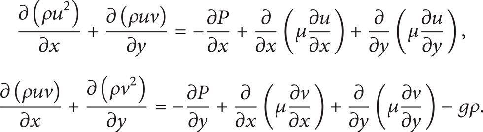
\begin{matrix} \frac{\partial (ρ u^{2})}{\partial x} + \frac{\partial (ρ u v)}{\partial y} = - \frac{\partial P}{\partial x} + \frac{\partial}{\partial x} (μ \frac{\partial u}{\partial x}) + \frac{\partial}{\partial y} (μ \frac{\partial u}{\partial y}), \\ \frac{\partial (ρ u v)}{\partial x} + \frac{\partial (ρ v^{2})}{\partial y} = - \frac{\partial P}{\partial y} + \frac{\partial}{\partial x} (μ \frac{\partial v}{\partial x}) + \frac{\partial}{\partial y} (μ \frac{\partial v}{\partial y}) - g ρ . \end{matrix}

(2)

The energy equation is

\frac{\partial (ρ h)}{\partial x} + \frac{\partial (ρ u v)}{\partial y} = \frac{\partial}{\partial x} (k \frac{\partial T}{\partial x}) + \frac{\partial}{\partial y} (k \frac{\partial T}{\partial y}) + q_{v},

(3)

where h is the enthalpy and q_v is the volumetric heat source.

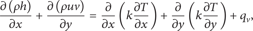
The buoyancy-driven flow regime of natural convection should be decided by the Rayleigh number, which can be viewed as the ratio of buoyancy and viscosity forces times the ratio of momentum and thermal diffusivities,

Ra = G r Pr = \frac{g β Δ t l^{3}}{ν^{2}} Pr = \frac{g β Δ t l^{3}}{a ν},

(4)

where Pr is the Prandtl number, g isgravity, l ischaracteristic length, a isdynamic viscosity, ν iskinematic viscosity, and β is thermal expansion coefficient.

Ra less than 10⁸ indicates a buoyancy-induced laminar flow [16], with transition to turbulence occurring over the range of 10⁸ < Ra < 10¹⁰.

2.2. Solution Method

To simplify the heat transfer model, several assumptions are used:

steady state;

2D heat transfer model;

the absorber plate temperatures are fixed and resulting heat losses are calculated.

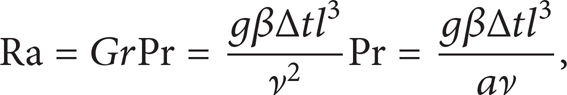
Notation for the cavity dimensions is shown in Figure 3. Fixed parameters in the modeling are shown in Table 1, and variable parameters are shown in Table 2.

Table 1:

Constant parameters sued in the simulation.

Constant parameter	Symbol	Value

Absorber plate width	W	160 mm
Side walls emissivity	ε_W	0.5
Glass window emissivity	ε_g	0.85
Glass window transmissivity	τ_g	0.95
Insulation thermal conductivity	λ_i	0.04 W/(m·K)

Table 2:

Variable parameters sued in the simulation.

Varied parameters	Symbol	Value

Cavity depth	h	50 mm, 100 mm, and 150 mm
Side wall inclination	θ	30°, 45°, and 60°
Insulation thickness	d	0 mm, 10 mm, 20 mm, and 30 mm
Ambient temperature	T _a	270 K, 280 K, 290 K, 300 K, and 310 K
Absorber plate temperature	T _P	100°C, 200°C, 300°C, and 400°C
Emissivity of selective absorption coating	ε_P	0.05, 0.1, 0.2, 0.3, 0.4, and 0.5

Figure 3:

Schematic of cavity geometry.

The heat transfer model is solved by the commercial CFD software Fluent 6.3, taking into account all heat transfer mechanisms: radiation, convection, and conduction. A 0.5 m × 0.5 m outer space is created for computing convection and radiation between the cavity and the environment. Heat transfer is fierce inside and around the cavity, so the grid is detailed there. Triangle mesh is used in the entire region, which is shown in Figure 4.

Figure 4:

Mesh of the entire region.

The absorber plate is modeled as isothermal surface. Surfaces of side walls, insulation, and glass window are modeled as combined convection/radiation boundary. The simulation model is laminar according to Ra number.

In this model, the glass window is semitransparent, so the discrete ordinates (DO) radiation model is chosen. All discretization is carried out using first order upwind. Air properties are modeled as piecewise linear. Minimum convergence criteria are set at 10⁻³ for continuity and velocity and 10⁻⁶ for DO and energy. First, 500-step iterations are carried out under default underrelaxation factors and then turn them down, proceeding 10000-step iterations, monitoring the temperature of outer surface of glass window, making sure there is no fluctuation.

3. Results and Discussion

3.1. Heat Loss Coefficient

When heat absorption and heat release reach a balance of the cavity receiver, as usualstating under steady state, the capacities that are absorbed and lost are equal:

q_{loss} = q_{a} = m C_{P} (T_{o} - T_{i}),

(5)

where m is the mass flow rate, T_i is the working fluid inlet temperature, and T_o is the working fluid outlet temperature.

Heat loss coefficient U_L is a key indicator of the thermal performance of the cavity receiver. As the U_L increases, the total heat lost increases. U_L is defined as

U_{L} = \frac{q_{loss}}{A_{P} (T_{P} - T_{a})},

(6)

where A_P is the area of absorber plate, namely, area of the side coated with absorbing coatings, T_P is the temperature of absorber plate, and T_a is the temperature of ambient air.

According to the literature [17], U_L can be predicted by the following empirical formula:

U_{L} = c \cdot {(T_{P} - T_{a})}^{d} .

(7)

3.2. Heat Loss Simulated Result

The heat loss coefficient based on absorber plate aperture was calculated as a function of the difference between average tube temperature and ambient air temperature; see Figure 5. Figures 6 and 7 show the velocity magnitude inside the cavity, temperature of the absorber plate is 400°C, and width is 160 mm. These two figures confirmed the convection heat transfer of inside walls through the air flow. Velocity near the side walls is the strongest among the inside area, the flow is enhanced when the cavity depth grows, and the biggest velocity occurs when cavity depth is 150 mm, which is 0.0821 m/s.

Figure 5:

Nonlinear curve fit of U_L (h = 100 mm, d = 20 mm).

Figure 6:

Contours of velocity magnitude inside the cavity for h = 50 mm.

Figure 7:

Contours of velocity magnitude inside the cavity for h = 150 mm.

Heat losses through glass window are higher than through insulation layer, which can be observed in Figure 8. With the rise of the temperature of absorber plate, the difference is getting more and more obvious. When the temperature of the absorber is 100°C, heat losses through glass window are 1.48 times of that through insulation, when the temperature of the absorber reaches 400°C, that is, 1.84. The radiation losses dominate the thermal losses inside the cavity as presented in Figure 9, and the radiation losses through the glass window occupy the most of the total heat losses.

Figure 8:

Schematic of heat loss versus T_P (h = 100 mm, W = 160 mm, and d = 20 mm).

Figure 9:

Schematic of heat loss versus T_P (h = 100 mm, W = 160 mm, and d = 20 mm).

Figure 10 shows the heat loss coefficient U_L versus the absorber temperature. U_L increases with the increase of the absorber temperature. When the temperature of the absorber plate is 100°C, U_L is 9.35 W/(m²·K); as to 400°C of the absorber plate, U_L is 17.21 W/(m²·K), and 84.1% is decreased.

Figure 10:

Schematic of U_L versus T_P (W = 160 mm, d = 20 mm).

We can also notice the influence of cavity depth h to the heat loss coefficient U_L from Figure 10. When the ambient temperature, insulation thickness, and the inclination of side walls are constant, U_L varied with cavity depth are small, but U_L with the 100 mm cavity depth are the smallest in general.

Hold other parameters' constant, such as width of absorber plate and cavity depth, and change the inclination of side walls; the influence is shown in Figure 11. U_L shows a downtrend with the increase of inclination of side walls; compared with U_L with the 30° inclination, 9% declination occurs with the 60° inclination of side walls; this is because areas of glass window and lateral wall surfaces are increased.

Figure 11:

Schematic of U_L versus θ (W = 160 mm, d = 20 mm, and h = 50 mm).

The insulation layer is an effective arrangement to minimize the heat losses through the cavity outer surface. We choose four insulation thicknesses for validating the influence of insulation: 0 mm, 10 mm, 20 mm, and 30 mm. The result is shown in Figure 12; as expected, the heat transfer coefficient decreases with the increase of insulation thickness. Heat losses coefficient with 10 mm insulation thickness is 58% lower than that of without insulation. But to continue increasing the thickness of insulation, the heat preservation effect improving is not obvious. Heat losses of the cavity with 30 mm insulation thickness only reduce by 2.2%, compared with 10 mm insulation thickness.

Figure 12:

Schematic of U_L versus d (W = 160 mm, h = 50 mm, and θ = 45°).

The main effect of glass window is to minimize the convection heat transfer between cavity inside and ambient air; the influence of glass window on total heat loss coefficient is shown in Figure 13. The effect of glass window is obvious; when cavity depth is 50 mm, 100 mm, and 150 mm, U_L of cavity with glass window has declined by 4.4%, 9.6%, and 10.8%, respectively. The concentrated solar beam causes an incidence angle on the outer surface of glass window that is greater than 0°, which means optical losses will be produced, so we should choose the glass window with high transmissivity and low reflectivity.

Figure 13:

Schematic of U_L versus h (W = 160 mm, d = 20 mm).

The turning point ofsolar thermal utilizations is the popularization and use of selective absorption coating, which has a high absorptivity (>0.9) and low emissivity (<0.1). Since the first presentation by the experts of Israel and America in 1954, much research has been done so far [9]. The selective absorption coating can work under 550°C, which solves the bottleneck of concentrated solar energy utilization. The influence of selective absorption coating to U_L is shown in Figure 14; U_L increases nearly linearly with the increase of selective absorption coating emissivity of absorber. When the coating emissivity ε_P is 0.05, U_L is 11.85 W/(m²·K), which is 47% lower than U_L with the 0.5 coating emissivity.

Figure 14:

Schematic of U_L versus ε_P (d = 20 mm, W = 160 mm, h = 50 mm, and θ = 45°).

The declination of ambient temperature will lead to the increase of heat loss (see the q_loss curve in Figure 15); this makes sense, but U_L declines with the increase of ambient temperature. As mentioned in Section 2 of this paper, U_L can be regarded as the heat transfer coefficient between the outer surface of the cavity and the ambient air; according to the Newton cooling law, the smaller the temperature difference, the larger the heat transfer coefficient. The influence of ambient temperature on U_L is small; when T_a increase from 270 K to 310 K, U_L just increases by 6.7%.

Figure 15:

q_loss and U_L versus T_a (d = 20 mm, W = 160 mm, h = 50 mm, and θ = 45°).

4. Conclusions

In this paper, a CFD performance prediction and optimum of the cavity receiver for linear Fresnel reflector concentrator have been made, considering the cavity configuration and other influence factors, and the effect on U_L is complex; main conclusions are as follows.

The most important factors which influence the heat loss coefficient are insulation and emissivity of selective absorption coating, which can reduce 58% and 47% of the heat loss coefficient, respectively; glass window plays the second position, which can reduce 10.8% of the heat loss coefficient at most when cavity depth is 150 mm. The influence of ambient temperature is small.

The heat loss coefficient shows a downtrend with the increase of inclination of side walls; the influence of cavity depth is negligible, which is consistent with the conclusion of Facão and Oliveira [18]. Among all the cavity models that are simulated in this work, the trapezoidal cavity with 100 mm cavity depth and 20 mm insulation thickness plays the best thermal performance.

Conflict of Interests

The authors declared that they have no conflict of interests related to this work.

Footnotes

Acknowledgments

This work was supported by the National Natural Science Foundation of China (Grant no. 51106091) and the Shandong University Innovation Foundations (Foundation no. 2012ZD018).

References

Kalogirou

S. A.

, “Solar thermal collectors and applications,” Progress in Energy and Combustion Science, vol. 30, no. 3, pp. 231–295, 2004.

Cable

R. G.

Cohen

G. E.

Kearney

D. W.

, and Price

H. W.

, “SEGS plant performance 1989–1997,” in Proceedings of the International Solar Energy Conference, pp. 445–452, June 1998.

Zhai

Dai

Y.-J.

, and Wu

J.-Y.

, “Investigation of concentrating solar photovoltaic/thermal system performance based on Fresnel lens,” Journal of Engineering Thermophysics, vol. 28, no. 5, pp. 725–728, 2007.

Velázquez

García-Valladares

Sauceda

, and Beltrán

, “Numerical simulation of a Linear Fresnel Reflector Concentrator used as direct generator in a Solar-GAX cycle,” Energy Conversion and Management, vol. 51, no. 3, pp. 434–445, 2010.

Häberle

Zahler

Lerchenmuller

, “The Solarmundo line focussing Fresnel collector. Optical and thermal performance and cost calculations,” in Proceedings of the International Symposium on Concentrated Solar Power and Chemical Energy Technologies, Zürich, Switzerland, 2002.

Nelson

D. T.

Evans

D. L.

, and Bansal

R. K.

, “Linear Fresnel lens concentrators,” Solar Energy, vol. 17, no. 5, pp. 285–289, 1975.

Feuermann

and Gordon

, “Analysis of a two-stage linear Fresnel reflector solar concentrator,” Solar Energy Engineering, vol. 113, p. 272, 1991.

Mills

, “Advances in solar thermal electricity technology,” Solar Energy, vol. 76, no. 1–3, pp. 19–31, 2004.

Morin

Platzer

Eck

Uhlig

Häberle

, and Berger

, “Road map towards the demonstration of a linear Fresnel collector using a single tube receiver,” in Proceedings of the 13th Solar PACES International Symposium, Seville, Spain, 2006.

10.

Mills

D. R.

and Morrison

G. L.

, “Compact linear fresnel reflector solar thermal powerplants,” Solar Energy, vol. 68, no. 3, pp. 263–283, 2000.

11.

Pino

F. J.

Caro

Rosa

, and Guerra

, “Experimental validation of an optical and thermal model of a linear Fresnel collector system,” Applied Thermal Engineering, vol. 12, pp. 1–9, 2012.

12.

Chemisana

and Ibáñez

, “Linear Fresnel concentrators for building integrated applications,” Energy Conversion and Management, vol. 51, no. 7, pp. 1476–1480, 2010.

13.

Han

, and Pei

, “Theoretical study of parabolic trough solar concentrator,” Acta Energiae Solaris Sinica, vol. 30, no. 9, pp. 1182–1187, 2009.

14.

Singh

P. L.

Sarviya

R. M.

, and Bhagoria

J. L.

, “Thermal performance of linear Fresnel reflecting solar concentrator with trapezoidal cavity absorbers,” Applied Energy, vol. 87, no. 2, pp. 541–550, 2010.

15.

Dey

C. J.

, “Heat transfer aspects of an elevated linear absorber,” Solar Energy, vol. 76, no. 1–3, pp. 243–249, 2004.

16.

and Ma

, “Numerical simulation of the closed cavity of high Rayleigh number laminar natural convection,” Journal of Huazhong University of Science and Technology, vol. 21, pp. 1417, 2004.

17.

Masterson

K. D.

, “Selective surfaces for solar-thermal conversion,” Journal of Solid State Chemistry, vol. 22, no. 1, pp. 41–49, 1977.

18.

Facão

and Oliveira

A. C.

, “Numerical simulation of a trapezoidal cavity receiver for a linear Fresnel solar collector concentrator,” Renewable Energy, vol. 36, no. 1, pp. 90–96, 2011.