
Abstract
Intervehicle communication gives vehicles opportunities to exchange packets within the limited radio range and self-organized in Ad Hoc manner into VANETs (Vehicular Ad Hoc Networks). However, due to issues such as the high mobility, insufficient market penetration ratio, and lacking of roadside units, connectivity is actually a big problem in VANETs. In addition, relying only on the direct connectivity in most of the previous works, say broadcasting which provides one-hop connections between nodes is far from the continuously growing application demands in VANETs, such as inter-vehicle entertainments, cooperative collision avoidances, and inter-vehicle emergency notifications. Therefore, the indirect connectivity from multihop forwarding is also a necessary complement especially for the case where direct connection is hardly achieved. In this paper, we define a new metric, that is, available connectivity, to consider both direct and indirect connectivity. After analyzing the statistical properties of direct and indirect connectivity in vehicular environment, the available connectivity is proposed and quantified for practical usage. Numerical results show that our available connectivity could provide correct and useful references for protocols design and performance improvements of different applications.
1. Introduction
Vehicular Ad hoc Networks [1–3] (VANETs) are distributed, self-organized communication networks composed of moving vehicles and are thus characterized by very high nodal mobility and limited degrees of freedom in the mobility patterns. The discussed IEEE 1609 Wireless Access in Vehicular Environments [4] (WAVE) draft is being developed for VANETs applications mainly considering safety-related scenarios, such as cooperative forward collision warning [5, 6] (CCW) systems, traffic signal violation warning [7] systems, and lane change warning [8] systems, and at the same time taking account of some requirements from nonsafety-related applications [9]. Indeed, all the above applications greatly rely on the packets exchange on reliable links and robust connections between vehicles. From this perspective, network connectivity becomes a fundamental and crucial issue to any practical application in VANETs. Regarding the node mobility, vehicles can not only depend on the direct one-hop broadcasting; they also need packets to be indirectly forwarded to the destinations through store-carry or multihop relays. However, it is worth noting that both direct and indirect connections are sometime hardly achieved especially during sparse communication environments such as the suburb highway or cases with low market penetration ratio [10]. As a result, the limited connectivity directly affects the possible speed at which information can be transported over a VANET and hence directly influence the up-to-datedness of wanted notifications which may result in accidents.
In summary, analysis to the connectivity is very necessary in VANETs. Actually, a number of models have been proposed in previous works such as stochastic process [11] based, Gaussian unitary ensemble (GUE) of random-matrix theory [12] based, and queuing theory [13] based and almost all their works discussed the connectivity with the famous three-phase traffic theory in which the fundamental relationship between traffic parameters on a road segment is given by the following equation:

where F, S, and K are the traffic flow, average speed, and traffic density, respectively. The influences on the connectivity from the above parameters can be disclosed from Figure 1. Before the state transforming point, at which packets begin to be queued in transceivers' sending buffers when the density of vehicles increases, the connectivity is intermittent and thus needs further studying to improve the performance. For the stage after the state transforming point, which is named the congestion flow state and depicted by dashed line, the connectivity could be basically guaranteed regarding the larger density. In that case, road is often jammed by vehicles very close to each other whereby the direct connectivity can be readily obtained. Accordingly, our research will focus on the free-flow state depicted by the solid line throughout our paper.

Relationship between basic parameters in the vehicle traffic theory.
The rest of the paper is organized as follows. Section 2 provides our research motivations and discusses the possible usages of the available connectivity in VANETs. Section 3 presents previous related works. Section 4 introduces our definition of the available connectivity, assumptions, and the statistical analysis of direct and indirect connectivity. Numerical results and performance evaluations are presented in Section 5. Our work is concluded in Section 6 followed by acknowledgments and cited references.
2. Motivations
“Connectivity” in Ad Hoc networks actually has a mature body of research but still absorbed lots of research interests in VANETs recently. With VANETs gradually stepping into our daily life, the connectivity has played an important role in many road applications to ensure driving safety and increase comfortableness. For instance, in CCW scenario, a good connectivity could help to avoid the chain collisions through disseminating warning notifications farther and quicker. In Figure 2, the red car crashed with the blue car and sent a CCW message. Then, car 1 could receive the CCW by direct connection and take brake in time to avoid crash. However, without the help of the indirect connection, that is, multi-hop forwarding in this case, car 2, and 3 may collide with the front car if the intervehicle distances are approaching the unsafe range [14]. In Figure 3, vehicles 2~5 could detect the front traffic jam by the messages store-carry-forwarded by vehicle 1 from the red sender. Therefore, owing to the indirect connectivity, they can beforehand enter into the auxiliary road to avoid the congestion and save time. In summary, the connectivity, direct or indirect, could provide more opportunities for vehicles to make their decisions wisely and safely and to achieve better driving experiences. Hence, a good definition of the connectivity or the metric to measure the connectivity is essential in VANETs.

CCW application scenario.
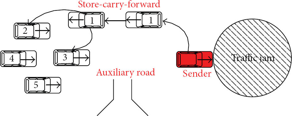
Traffic jams avoidance.
In our work, we define the connectivity as the probability of connections which could be achieved directly or indirectly. Numerical results show that our definition can explore the potential transmission opportunities for vehicles especially in the safety-related applications context. The connection possibility is discussed through statistical analysis in terms of either connected durations or inter-vehicle distances. To reflect the high dynamics of the connectivity due to different mobility patterns, we also introduce the influence of velocity into our work.
Indeed, a wise definition of the available connectivity can practically make many otherwise complex problems easy. For example, to design an admission control strategy in VANETs, the available connectivity could provide important references for the connectivity improvement by giving the specific time or location at which the vehicles may be admitted into. In addition, to evaluate the performance of emergency-related applications, the available connectivity could roughly work out the delivery ratio of emergency notifications from given vehicles. On the other hand, to make the emergency notifications spread faster and further, the available connectivity could also be taken as a better criterion for relays selection. Besides, to route the packets based on the available connectivity, the throughput can be improved and the backup multiple paths may be simultaneously figured out whereby transmission robustness could be guaranteed. In a dense network, available connectivity may also be able to offer a reference for the threshold of packet generation rate to maintain sufficient connectivity but not make the overall network congested. In summary, along with the available connectivity, a plethora of works now can be implemented to improve the safety, comfortableness, and efficiency in VANETs.
3. Related Works
Although connectivity analysis is a classical issue in wireless communication networks, it is now still a hot topic in VANETs regarding the recently increasing research activities [15–17]. In my point of view, the connectivity research in VANETs can be generally classified into two categories: one for investigating the lifetime properties of connected links or paths; another via the measurement of inter-vehicle distances.
Researches on lifetime properties mainly focus on the statistical analysis of the connection duration. In [11], the authors discussed the connection duration expression in detail considering the velocity vectors with yaw angles. Their numerical results found that high relative velocities impose a hard task on some cooperative maneuvers including underlying routing protocols. However, even the short connection duration is still enough for emergency notification scenarios. In [18], the connection duration between two adjacent vehicles was figured out, given their speeds, directions, and the radio ranges. According to the calculated connection period expression, an admission control strategy is proposed to determine whether the next vehicle is allowed to be injected into the current traffic flow without interrupting the ongoing connections. In [19], metrics for evaluating nodal connectivity in VANETs had been presented considering the different nodal mobility patterns. The connection period distribution was characterized by average duration of the k-hop path existing between any two nodes. They also showed by simulation that multi-hop paths have much poorer connectivity performance than the single-hop one in VANETs.
Researches on the connectivity through inter-vehicle distances attempt to disclose the relationship between the connectivity and the distance which is defined as the length of the connected path. In [11], the distance distribution had been expressed by a tuple (
4. The Connectivity Analysis in VANETs
4.1. The Analytical Model and Definitions
As we have stated before, the connectivity in the free-flow state is worth studying in view of its uncertainty and scarcity. Thus, in this section, we introduce a highway as our discussing objective where vehicles form a free-flow state traffic with lower distribution density. In our analysis, an equipped vehicle is taken as a node for simplicity. The discussed scenario is plotted in Figure 4, where all cars drive on a single lane represented by a line. We assume that

The analytical model used for highway and the vehicles traffic follows Poisson arrival process.
Definition 1.
Define the connectivity of two nodes as
Definition 2.
Let i be the farthest node which can communicate with
X is a variable representing the distance between
We suppose that two nodes are connected if they are falling into the radio range of each other and the disconnection due to collisions or asymmetrical channel conditions is not taken into account.
4.2. The Statistical Model with Constant Radio Range Setting
In this section, we discuss the connectivity when all nodes choose the same constant radio range, that is, R. We model the one-dimension highway as an

The relationship between M/D/∞ system and highway model.
We investigate

where μ is the average speed and σ is the standard deviation of velocity. We also introduce a metric, that is, speed factor, to reflect the impact of velocity on the inter-vehicle distances and the resulted connectivity.
Definition 3.
A is defined as the speed factor with unit hour/km as

where


For a PDF curve of a normal distribution, the region corresponding to the x-axis coordinate ranging from
With the above definitions and assumptions, the expression of connectivity with constant radio range setting could be given as follows.
Theorem 4.
For the case where vehicles all have the same constant radio range, the connectivity could be deduced as

where

Proof.
Let

where

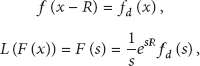
where
Therefore, we have the following equations:
where
Based on Definition 2 for an end node, the connectivity of any node at x is

and its Laplace transform is

With above equations, (12) can be rewritten as
Actually, in [13], the CDF expression of the inter-vehicle distance is given by

and the average inter-vehicle distance is written as

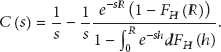
Thus, with (12) and (14), we have

Applying an inverse Laplace transforming [30] to (16), we have the expression of
Remark 5.
Remark 6.
If a node is exactly located at
Remark 7.
The above remarks also validate Theorem 4. To understand this theorem in depth, we also explore some connectivity-related statistical properties including the probability that a given node is isolated, the area that a sent message may cover, and the probability of the number of connected nodes. We also classify the connected nodes into two categories by relaying hops between them and analyzing the corresponding connectivity.
(1) Probability that a Given Node Is Isolated. The probability that a given node is isolated, denoted by
Theorem 8.
The isolation probability is given by

For a node at x,
(2) The Area that a Sent Message May Cover. We discuss the area that a sent message from the reference node can cover. The single and multi-hop cases are both considered. Generally, this characteristic can also be evaluated with coverage probability. Here, we use the expectation to show the average value in general case. Because the system is initially assumed not empty, the mathematic expectation could be given by the following theorem.
Theorem 9.
The expectation of the coverage area for a message sent from the reference node is

where
Proof.
Based on [27], we can obtain the following equations for different system initial conditions. Consider

Corollary 10.
If both sides of the discussed node are considered, (18) could be rewritten as

where
(3) Probability of the Number of Connected Nodes. The node which can reach the reference node is called a connected node. Here we discuss the possible number of the connected nodes, that is,
Theorem 11.
The Probability Mass Function (PMF) of

where
Proof.
We first focus on
The PMF of

The result for

Simplify the above equation and then the result can be rewritten as (21).
Theorem 12.
The tail probability of

Proof.
According to (21), we have

In addition, the probability that at most k nodes are connected is

The probability generating function (PGF) of

And the expected value of

Substituting (14) into (28), we obtain

Corollary 13.
The expectation of

Let Q be the probability lower bound when the number of connected nodes is

For a given Q and

Actually, the radio range is together determined by the transmission power

Similarly, the equation for Q considering both sides is

Corollary 14.
The critical range

According to (32) and (33), the connectivity could be flexibly controlled via radio range adjustment.
(4) Two Kind of Connected Nodes
Definition 15.
The connected nodes can be classified into two categories: (1) nodes within the radio range of the reference node, which is denoted by
An

In the same way, the

And the expectation of

The
Theorem 16.
The PMF of

Proof.
From (22), (26), and (36), for

where

When

And the PDF of

Taking Laplace transform to the above equation, we have
According to the independence of inter-vehicle distances, the following equation can be derived as

Then the PDF of

where
Meanwhile, the following conditional probability can be obtained as

With (22), (43), (46), and (47), we have

When

Then, the PMF of
Corollary 17.
The PMF of

Proof.
Through (51), we have

Corollary 18.
The expectations of

We define

4.3. Statistical Model Considering Random Radio Range
If the channel fading is taken into account, the reachable radio range should be reconsidered. Thereupon, the connectivity will also need reexamination. For notion simplicity, we name such variable “radio range” as ERR (equivalent radio range). The
The PDF of the busy period is [27]

where

Note that, in our work, route selection is based on the shortest path algorithm. And (54) corresponds to the case that nodes at
Hereinafter, we define
Theorem 19.
The connectivity for the random radio range case can be expressed as

where a denotes the distance between the end node and its nearest relay.
Proof.
We assume that there are m connected nodes on
According to the definition of X, then

The connectivity between the reference node and a given node with

To reflect the general fading types in vehicular environment, the Rayleigh and lognormal shadowing are introduced in our work. According to [31–33], the corresponding CDF and expectations of the radio range for the above fading models are as follows.
Lemma 20.
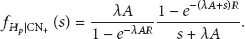
The PDF and average ERR of Rayleigh fading are


Lemma 21.
The PDF and average ERR for lognormal shadowing are


where

Note that one just discusses the cases under free-flow state, say λ is generally very small. Then, in a Rayleigh fading channel, the pass loss factor could be taken as a constant during the transmission of a frame. Indeed, when λ becomes very large, the above assumption may fail in some cases.
Similar to the analyzing procedure when the radio range is constant, one also investigates some statistical characteristics for random radio range case, that is, probability that a given node is isolated, the area that a message may cover, the probability of the number of connected nodes, and its value for
(1) The Probability That a Given Node Is Isolated. For a fading channel, the number of nodes within R is Poisson distributed with parameter

(2) The Area that a Transmitted Message May Cover. Based on [30], we know, the computational complexity of (56) is very high. However, by [27], the expectation value of the coverage area for a sent message is

where

The expectations for the area on the right and both sides are, respectively,

(3) The Probability of the Number of Connected Nodes. As stated in the corresponding parts for constant radio rage case,

Because the radio range is a stochastic variable under a random channel, by (69), the number of connected nodes is mainly determined by the nodes with smaller ranges.
If we focus on the nodes which are within the radio range of

With (70), the PMF, CDF, and expectation expressions could be derived in theory. However, the procedures are actually very computationally complex. Owing to the works by [34, 35], the above statistics could be deduced in a simple way. Suppose that the vehicular arrival process is a Markovian arrival process (MAP) and it is stationary, ergodic, and nonempty. Without loss of generality, we assume that the arrival traffic flow size in MAP is one [27] and nodes enter into this system one by one.
According to [36],

and the result considering both sides is

(4) Two Kinds of Connected Nodes. Let

For the number of nodes out of the radio range of

where
4.4. Available Connectivity
The connectivity
Definition 22.
Available connectivity is defined as a metric to measure the connection possibility for a given node considering the contributions on connections from others.
Let i be an equipped vehicle running on a one-dimensional highway.
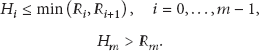
Limitation I.

Limitation II.

where
To make our work practical, we discretize the time continuous variable
Definition 23.
Available connectivity includes two kinds of dissemination ways, say the direct and indirect. Namely, available connectivity is equal to the arithmetic sum of the direct connectivity and indirect connectivity.
Direct connectivity: the connection probabilities between a given node and its Indirect connectivity: the connection probabilities between a given node and its
Theorem 24.
The available connectivity of node i at time T is

where
Similarly, we have

where

where
With (77) and the definition of our available connectivity, we know that the number of hops influences the connection performance significantly. For different applications, the requirements of hop bounds are variously depending on the delay limitation, information generation frequency, energy efficiency, and so forth. Considering the high dynamics in VANETs, larger hops may correspondingly incur intolerable delays, thus resulting in the service failure especially for emergent events. Therefore, a small hop bound is acceptable in VANETs.
When using the shortest path route selection algorithm, the following two corollaries hold.
Corollary 25.
For the case that the radio range is a constant, Limitation I could be rewritten as

thus
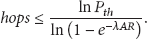
Corollary 26.
Similarly, we can derive out the corresponding expression for the case where the radio range is a random variable depending on channel fadings. Consider

With (82), the probability upper bound of the number of hops could be deduced.
5. Numerical Results
In this section, we will evaluate the performance of our proposed metric and investigate its feasibility and effectiveness with different simulation settings.
5.1. The Relationship between the Connectivity and R, λ, and A
According to (6) and (56), it is noted that the radio range R, the equipped vehicle arrival rate λ, and the speed factor A all have influences on the connectivity. In [37], the author provided some typical values for the expectation and standard deviation for vehicular speed on highway which follow the normal distribution as listed in Table 1. We will also use these settings in our later simulations.
Normal-speed statistics.

The speed factor A is actually a function of μ and σ. Thus, we will firstly analyze the impact of μ, σ on A. The result is plotted in Figure 6. It is noted that the speed factor decreases when the mean of the velocity increases. In addition, the standard deviation has only a very limited influence on A. For σ, a great increasing of it could only slightly augment the speed factor.

The relationship between speed factor A (hour/km) and the expectation μ (km/hour), the standard deviation σ (km/hour).
The connectivity performance when the radio ranges of all nodes are the same constant is showed in Figure 7. In this simulation scenario, we placed 31 vehicles along a one-dimensional highway and investigated the resulted connectivity for a given node at x with different R (m), λ (vehicles/hour), and A (hour/km).

Connectivity versus x (m) with the radio range R (m), vehicle arrival rate λ (vehicles/hour), and speed factor A (hour/km) changing when all the nodes use the same constant radio range.
From Figure 7, it is noted that when
As a result, it is noted that the variation of the radio range R will mainly influence the connectivity performance compared to other factors. With this conclusion, a critical radio range could be calculated for transmitting power saving consideration and applied to scenarios with determined connectivity requirements.
5.2. The Isolation Probability
The probability that a given node is isolated plays an important role in VANETs. Usually, it can be used for algorithms concerning clustering forming, relay selection, routing metric, and so forth. To reflect its influence on connectivity, the isolation probability is shown in Figures 8 and 9 based on (17) and (65), where Figure 8 corresponds to the constant radio range case and Figure 9 for the random radio range case. It is noted that in Figure 8, R is still the main influential factor to

The isolation probability considering nodes on both sides for the constant radio range case.

The isolation probability
For random radio range case, we compare the isolation probability under the deterministic, Rayleigh, and shadowing fading channel, respectively, as shown in Figure 9. From this figure and (33), (61), and (63), we notice that the Rayleigh shows the worst performance of
5.3. The Number of Connected Nodes
Based on Theorem 16 and (14), the average tail probability of the number of connected nodes is plotted in Figure 10 for the constant radio range case. It is noted that the speed factor, arrival rate, and radio range all greatly influence the average tail probability. A smaller A, which corresponds to a larger average speed, will decrease the probability of vehicles forming a bigger cluster. The reason is that high mobility will make the network more dynamic and links unstable. As for the arrival rate λ, it seems to be in positive proportion to the average tail probability. In addition, among the three influential factors, radio range still contributes the most, which is consistent with the results from Figures 7 and 8.

The average tail probability of the number of connected nodes for the constant radio range case.
Figure 11 depicts the corresponding average tail probability of the random radio range case. We set

The average tail probability of the number of connected nodes on the right of the reference node for the random radio range case.
5.4. Available Connectivity
In this subsection, we will investigate the performance of our introduced available connectivity metric. For simplicity, the threshold of connectivity and
The performance for the constant radio range case is shown in Figure 12. When setting the arrival rate λ to 500 vehicles/hour, speed factor A to 0.008672 hour/km (corresponding to

Available connectivity versus t (second) within 80 seconds for the case of constant radio range.
The available connectivity in random fading channels are plotted in Figures 13 and 14, where we set

Available connectivity versus t (seconds) within 80 seconds for the random radio range case.

The impact of hop bounds on the available connectivity under random fading channels.
To show the impact of hop bounds on the available connectivity, the performance from different hop bounds and channel fadings is plotted in Figure 14. Note that the upper bound of hops in Figure 13 is adaptively adjusted according to the average radio range. Because the hop bound is decided by application requirements, we introduce different settings including 5 (correspond to emergency case), 10, and 20 (corresponding to the delay tolerable services) in Rayleigh fading channel and lognormal shadowing channel. As shown in Figure 14, it is noticed that the different hop bounds settings greatly influence the available connectivity and a larger hop bound means a higher available connectivity. Thereupon, hop bounds should also be taken into consideration when designing different applications in VANETs.
6. Conclusion
In this paper, a useful metric, that is, available connectivity has been introduced in VANETs. Our proposed available connectivity comes not only from direct connections from neighbors, but also from the indirect links by multi-hop relay. The elaborate investigations of the related statistical properties of the connectivity have been given to reflect the influential factors and give the important references for applications design. Numerical results show that our proposed available connectivity has many potential relationships with network parameters and may provide important references for future protocols design in VANETs.
Footnotes
Acknowledgments
This work was supported by the National Natural Science Foundation of China (61201133, 61172055, and 61072067), Xian Municipal Technology Transfer Promotion Project (CX12178(6)), the Fundamental Research Funds for the Central Universities (K5051301011), the Postdoctoral Science Foundation of China (20100481323), the Program for New Century Excellent Talents (NCET-11-0691), the “111 Project” of China (B08038), and the Foundation of Guangxi Key Lab of Wireless Wideband Communication & Signal Processing (11105).