Sage Journals: Discover world-class research

Abstract

Blood is in fact a suspension of different cells with yield stress, shear thinning, and viscoelastic properties, which can be represented by different non-Newtonian models. Taking Casson fluid as an example, an unsteady solver on unstructured grid for non-Newtonian fluid is developed to simulate transient blood flow in complex flow region. In this paper, a steady solver for Newtonian fluid is firstly developed with the discretization of convective flux, diffusion flux, and source term on unstructured grid. For the non-Newtonian characteristics of blood, the Casson fluid is approximated by the Papanastasiou's model and treated as Newtonian fluid with variable viscosity. Then considering the transient property of blood flow, an unsteady non-Newtonian solver based on unstructured grid is developed by introducing the temporal term by first-order upwind difference scheme. Using the proposed solver, the blood flows in carotid bifurcation of hypertensive patients and healthy people are simulated. The result shows that the possibility of the genesis and development of atherosclerosis is increased, because of the increase in incoming flow shock and backflow areas of the hypertensive patients, whose WSS was 20~87.1% lower in outer vascular wall near the bifurcation than that of the normal persons and 3.7~5.5% lower in inner vascular wall downstream the bifurcation.

1. Introduction

Blood is a suspension of different cells including red blood cells, white blood cells, and platelets in plasma. Red blood cells occupy the great portion (98%) of these cells and determine the rheology of blood. In this sense, blood is a complex non-Newtonian fluid with yield stress, shear thinning, and viscoelastic properties. With the development of computational biomechanics, some researchers [1 –5] have carried out numerical simulations of blood flow. However, whether the blood can be treated as Newtonian fluid or not in the numerical simulation is still worthwhile to discuss. Several researchers indicated that the non-Newtonian behavior of the blood in great vessels has little influence on the local flow characteristics [6 –8]. Nevertheless, other researchers [9 –11] insist that it is of significant influence. In a word, the blood rheology has strong impact on the hemodynamics, and it is necessary to describe blood flow by proper non-Newtonian model. Considering the non-Newtonian characteristics, a variety of non-Newtonian models, such as Cross, Power Law, Bingham, and Carreau modes, can be found in commercial CFD software. However, Casson model widely used [12 –15] over a large range of shear rates [16 –18] for the studies of blood rheology was not implemented by commercial software. In this study, the Casson model will be adopted to develop non-Newtonian flow solver.

Clinical studies indicate that many cardiovascular diseases, such as atherosclerosis and aneurysm, often occur in coronary arteries, carotid artery bifurcation, and abdominal aorta, where the geometrical structures of the flow region are complex because of the bifurcation and curvature of the vessels. For numerical simulation, the unstructured triangle grid has obvious advantages in the discretization of this complex flow region because of the flexibility in element meshing and strongly adaptability to complex region [19, 20]. Consequently, we will develop an unsteady solver on unstructured grid for the simulation of non-Newtonian blood flow with Casson model.

The carotid artery bifurcation is known to be one of the favoured sites for the genesis and development of atherosclerotic lesions. The relation between the hemodynamic factors (e.g., shear stress and the localized development of atherosclerosis) has been studied. Chen and Lu [21, 22] treated the blood as a Carreau-Yasuda fluid and investigated the influence of the shear thinning behavior and pulsatile property of blood on wall shear stress (WSS). Perktold et al. [23, 24] numerically simulated the blood flow in different carotid artery bifurcation models under pulsatile flow condition using a pressure correction finite element method. By treating the blood as a Newtonian fluid, they compared the velocity profile and the distribution of WSS with the experiment results from Ku and Giddens [25]. Jou and Berger [26] assumed the flow in the carotid bifurcation is Newtonian fluid in a rigid vessel and simulated the steady and unsteady flows using the artificial-compressibility method. Considering the blood as Newtonian, Casson, and hybrid fluids, Fan et al. [8] investigated the differences of the velocity profiles and the WSS distributions in a carotid artery bifurcation model using FLUENT 6.0. However, the computational investigation of blood flow in carotid artery bifurcation under normal and abnormal conditions, such as under hypertension [27], is still rare. The blood flow of other vascular tissue under hypertension has been studied using computational fluid dynamics. Gleason and Humphrey [28] presented a quantitative evaluation of the aortic wall stresses under systolic hypertension by using the spiral CT imaging and computational structural analysis. They detected the vulnerable high stressed regions under different values of systolic blood pressure and the resultant risk of rupture. Vasava et al. [29] investigated the blood flow in idealized model of human aortic arch under hypertension using finite element method. The results have shown that hypertension causes lowered local wall shear stresses which made the risk of atherosclerosis increased. Tang et al. [30] used a combined MRI and computational fluid dynamics approach to quantify flow features and WSS in pulmonary arterial hypertension (PAH) patients. They found WSS was significantly lower in the proximal pulmonary arteries of PAH patients compared to controls. Therefore, non-Newtonian blood flow in the carotid artery bifurcation under normotension and hypertension conditions will be simulated by the proposed solver.

This study consists of three parts. The first part presents a steady solver for non-Newtonian fluid flow by SIMPLE algorithm on unstructured collocated grid generated by our Delaunay triangulation method [31]. The sudden expansion flow is adopted to confirm the validation of Casson fluid flow algorithm and the flow in a T-type bifurcation is used to indicate the necessity of treating the blood as Casson fluid. The second part presents an unsteady non-Newtonian solver on unstructured grid. The lid-driven polar cavity flow starting from rest is adopted to validate the unsteady solver. The last part of this study focuses on the differences of blood flow under normotension and hypertension conditions in a carotid artery bifurcation using the proposed solver.

2. Steady Solver on Unstructured Grid

In light of the advantages of unstructured grid for the complex flow region discretization, a steady solver on unstructured grid is developed in this section.

2.1. Steady Solver for Newtonian Fluid

The incompressible SIMPLE algorithm is used for the velocity and pressure coupling [32]. The finite volume method is adopted to discretize the momentum equation, and the collocated grid system is used to arrange variables [33]. The momentum interpolation method proposed by Rhie and Chow [34] is adopted to eliminate the irrational pressure field in collocated grid.

The solving process contains two parts: the solution of the flow field and the correction of the pressure using the process of “guess correction.” The iteration is alternatively completed for solving the velocity and pressure until the simulation is convergent.

2.1.1. Solution of Flow Field

For laminar of Newtonian fluids, the planar steady incompressible flow can be described by the following general model of the governing equation:

div (ρ u ϕ) - div (λ_{ϕ} g r a d ϕ) = Q_{ϕ},

(1)

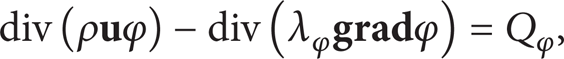
where φ is the generalized variable which can represent the velocity u and v, λ_φ is the generalized diffusion coefficient, ρ is the constant density, and Q_φ is the generalized source term.

In triangular cell P₀, the governing equation is integrated in space. Then the integral form of the governing equation can be gotten as follows:

\sum_{j = 1}^{3} \int_{S_{j}} (ρ ϕ u - λ_{ϕ} \nabla ϕ) \cdot d S = \int_{V_{P_{0}}} Q_{ϕ} d V,

(2)

where S_j is the area vector at cell interface, whose value is the length of the cell interface and direction is vertically outward as shown in Figure 1(a). V_{P
₀} is the volume of the cell P₀.

Figure 1:

Variables arrangement in unstructured triangular grid. (a) Generalized variable at the cell P₀ interface; (b) positional relationship between the cell and the interface.

For the convective flux,

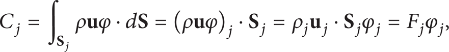
C_{j} = \int_{S_{j}} ρ u ϕ \cdot d S = {(ρ u ϕ)}_{j} \cdot S_{j} = ρ_{j} u_{j} \cdot S_{j} ϕ_{j} = F_{j} ϕ_{j},

(3)

where F_j denotes the flux at the cell interface gotten from the interface velocity (u_j) and j denotes the generalized variable at the cell interface, as shown in Figure 1(b). Using the momentum interpolation method, the interface velocity, u_j, is used for eliminating the irrational pressure field in the iteration:

u_{j} = (ω_{P_{0}} u_{P_{0}} + ω_{P j} u_{P j}) + \frac{1}{2} [{(\frac{V}{a_{0}})}_{P_{0}} + {(\frac{V}{a_{0}})}_{P_{j}}] \cdot [\frac{1}{2} (\nabla P_{P_{0}} + \nabla P_{P_{j}}) \cdot \frac{d_{j}}{| d_{j} |} - \frac{P_{P_{j}} - P_{P_{0}}}{| d_{j} |}] \frac{S_{j}}{| S_{j} |},

(4)

where d_j is the distance vector from node P₀ to P_j and u_{P
₀} is the velocities at node P₀.

For the diffusion flux,

D_{j} = - \int_{S_{j}} λ_{ϕ} \nabla ϕ \cdot d S \approx - λ_{ϕ j} \nabla ϕ_{j} \cdot S_{j},

(5)

where ∇ φ_j is the average value of the source term in the cell.

Source term is treated by local linearization method:

\int_{V_{P_{0}}} Q_{ϕ} d V = Q_{ϕ}^{P_{0}} V_{P_{0}},

(6)

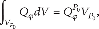
where Q_φ^{P
₀} is the average value of the source term in the cell.

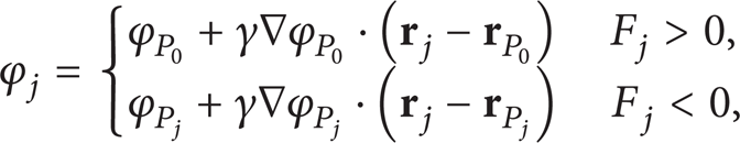
As long as the variable at the cell interface φ_j and its gradient ∇ φ_j are all obtained, the discretization equation is also achieved. The hybrid scheme of first-order difference scheme and central difference scheme is adopted to compute the variable φ_j:

ϕ_{j} = {\begin{cases} ϕ_{P_{0}} + γ \nabla ϕ_{P_{0}} \cdot (r_{j} - r_{P_{0}}) F_{j} > 0, \\ ϕ_{P_{j}} + γ \nabla ϕ_{P_{j}} \cdot (r_{j} - r_{P_{j}}) F_{j} < 0, \end{cases}

(7)

where r_j – r_{P
_j} is the distance vector from node P_j to the intersection point j as shown in Figure 1(b) and γ is the hybrid scheme factor. For the gradient of the variable at the cell interface, the central difference scheme is used:

\nabla ϕ_{j} = ω_{P_{0}} \nabla ϕ_{P_{0}} + ω_{P j} \nabla ϕ_{P j},

(8)

where $ω_{P_{0}} = - ((r_{j} - r_{P_{j}}) / d_{j})$ , $ω_{P_{j}} = (r_{j} - r_{P_{0}}) / d_{j}$ , and ∇ φ_{P
₀} is the gradient of the variable at node P₀. For the gradient of the variable at node P₀ in (8), Gauss' formula is used to accelerate the convergence:

\nabla ϕ_{P_{0}} = \frac{1}{V_{P_{0}}} \sum_{j = 1}^{3} ϕ_{j} S_{j} .

(9)

From the discretization above, the discretization model of the governing equation can be expressed as follows:

a_{0} ϕ_{P_{0}} = \sum_{j = 1}^{3} a_{j} ϕ_{P_{j}} + b_{0},

(10)

where

\begin{matrix} a_{0} = \sum_{j = 1}^{3} a_{j}, \\ a_{j} = \frac{λ_{ϕ_{j}}}{{| d_{j} |}^{2}} (d_{j} \cdot S_{j}) + \max (- F_{j}, 0), \\ b_{0} = \sum_{j = 1}^{3} λ_{ϕ} [\nabla ϕ_{j} - (\nabla ϕ_{j} \cdot \frac{d_{j}}{| d_{j} |}) \frac{d_{j}}{| d_{j} |}] \cdot S_{j} + \sum_{j = 1}^{3} γ \nabla ϕ_{j} \cdot [- (r_{j} - r_{P_{0}}) \max (F_{j}, 0) + (r_{j} - r_{P_{j}}) \max (- F_{j}, 0)] + Q_{ϕ}^{P_{0}} V_{P_{0}} . \end{matrix}

(11)

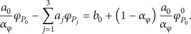
For the convergence of nonlinear iteration, the discretization equation is treated advantageously by the application of relaxation methods with the relaxation factor α_φ:

\frac{a_{0}}{α_{ϕ}} ϕ_{P_{0}} - \sum_{j = 1}^{3} a_{j} ϕ_{P_{j}} = b_{0} + (1 - α_{ϕ}) \frac{a_{0}}{α_{ϕ}} ϕ_{P_{0}}^{0} .

(12)

2.1.2. Correction of Pressure

For SIMPLE solver, the constructing and solving the pressure correction is necessary. Similar to the pressure correction in structured grid, the velocity at cell interface must satisfy the continuity equation in each iteration, so that substituting the corrected velocity ( $u_{j}^{*}$ ) at cell interface which includes the correction pressure (P_{P
₀}′)

u_{j}^{*} = u_{j} - \frac{1}{2} [{(\frac{V}{a_{0}})}_{P_{0}} + {(\frac{V}{a_{0}})}_{P_{j}}] \frac{S_{j}}{| d_{j} | | S_{j} |} (P_{P_{j}}^{'} - P_{P_{0}}^{'})

(13)

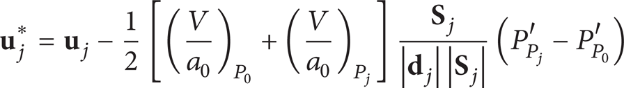
into the continuity equation, we can obtain the equation of the correction pressure:

a_{0}^{P} P_{P_{0}}^{'} = \sum_{j = 1}^{n} a_{j}^{P} P_{P_{j}}^{'} + b^{P},

(14)

where

\begin{matrix} a_{0}^{P} = \sum_{j = 1}^{3} a_{j}^{P}, \\ a_{j}^{P} = - ρ \frac{1}{2} [{(\frac{V}{a_{0}})}_{P_{0}} + {(\frac{V}{a_{0}})}_{P_{j}}] \frac{| S_{j} |}{| d_{j} |}, \\ b^{P} = \sum_{j = 1}^{3} F_{j} . \end{matrix}

(15)

Using P_{P
₀}′, the flow field and the pressure field of the current iteration step can be corrected:

\begin{matrix} P_{P_{0}}^{*} = P_{P_{0}} + α_{P} P_{P_{0}}^{'}, \\ u_{P_{0}}^{*} = u_{P_{0}} - \frac{V_{P_{0}}}{α_{0}} \nabla P_{P_{0}}^{'}, \end{matrix}

(16)

where α_P is the relaxation factor of the pressure.

2.1.3. Discretization of Boundary Condition and Convergence Conditions

The inlet is set as the velocity boundary where the velocity profile is assumed to be developed and parabolic. The output satisfies the second Neumann boundary and the other walls are set as nonslip boundaries.

The convergence conditions are the local and whole conservation of mass. The local conservation of mass is that the maximum absolute value of margin of continuity equation in all cell point is less than a certain value. The whole conservation of mass is that margin sum of continuity equation in all cells is less than another certain value. When the local and whole conservations of mass are satisfied simultaneously, the convergence condition is satisfied and the result in the current step is convergent.

2.2. Steady Solver for Non-Newtonian Fluid

Blood is a typical non-Newtonian fluid and can be described well by the Casson equation over a wide range of shear rate. To simulate the non-Newtonian fluid flow, a non-Newtonian fluid solver based on steady SIMPLE solver is developed.

Over a wide range of shear rate, blood can be described by the original constitutive equation for Casson fluid as follows [35]:

\sqrt{τ} = \sqrt{τ_{y}} + \sqrt{μ_{y} γ},

(17)

where τ is the shear stress, γ is the shear strain rate, γ = ∇ u + ∇ u^T, τ_y and μ_y are the yield stress and the Casson viscosity or the asymptotic apparent viscosity, respectively, which are correlated with hematocrit, and all models describe blood at a hematocrit of 45% in the paper. The difficulty for the implement of Casson model in numerical simulation is its discontinuous nature. Adopting a method used to overcome a similar singularity in a Bingham plastic fluid [36], a modified continuous version [12] can be used:

τ = {[\sqrt{μ_{\infty}} + \sqrt{\frac{τ_{y}}{| γ |}} (1 - e^{- \sqrt{m | γ |}})]}^{2} γ,

(18)

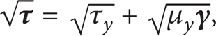
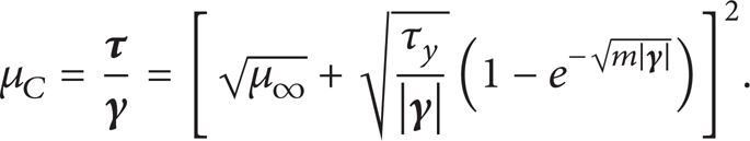
where μ_∞ is the asymptotic apparent viscosity and m is the model constant. Pham and Mitsoulis [37] proved that (18) can approximate the Casson model well when m > 100. From (18), it is known that the shear stress is a complex function of the shear strain rate related to the current solving velocity. So if the shear stress is involved directly in the discrete process, the simulation will be very complicated and the computation cost is expensive. In view of this, we suggest to use the apparent viscosity of the non-Newtonian fluid to replace the Newtonian fluid viscosity, which can avoid the complexity caused by direct discretization of the shear stress. The simplified solution for Casson fluid in this study can be used for all non-Newtonian fluids which can be modelled as τ = μ(|γ|)γ. The detailed process is shown in the following.

λ_φ in (1) is the viscosity of Newtonian fluid. When blood is assumed to be non-Newtonian fluid, λ_φ will be replaced by its apparent viscosity. The apparent viscosity for the Casson model can be defined as follows from the transformation of (18):

μ_{C} = \frac{τ}{γ} = {[\sqrt{μ_{\infty}} + \sqrt{\frac{τ_{y}}{| γ |}} (1 - e^{- \sqrt{m | γ |}})]}^{2} .

(19)

In solving process, the apparent viscosity μ_C can be calculated by the velocity field obtained from previous iteration to avoid the complexity of the discrete process and then be used to complete the current iteration. Substituting μ_C into (1), the modified governing equations are applicable for Casson fluids. Introducing the reference velocity U_∞ and reference length l, we can obtain $Bn = τ_{y} l / μ_{\infty} U_{\infty}$ . Here Bn is the Bingham number standing for the ratio of yield stress to viscous force, which is an important dimensionless number to describe non-Newtonian characteristics. The Reynolds number can be defined as $Re = ρ U_{\infty} l / μ_{\infty}$ .

In this way, the discretization of convective flux and source term can refer to the method for Newtonian fluid, and then the computation can be completed by steady solver on unstructured collocated grid.

2.3. Validation of the Non-Newtonian Model in Steady Solver

Numerical results for non-Newtonian fluid flow through a sudden expansion and steady blood flow in T-type bifurcation are presented below. The simulation of non-Newtonian fluid flow through a sudden expansion tests the validity of the treatment of the shear stress and viscosity in non-Newtonian SIMPLE solver, and the calculation of steady blood flow in T-type bifurcation validates the feasibility and necessity of Casson model in blood flow.

2.3.1. Non-Newtonian Fluid Flow through a Sudden Expansion

The geometry of the suddenly expanding channel is shown in Figure 2. It can be divided in two parts, namely, the inlet section and the outlet section, the heights of which are h and H. The expansion ratio, defined as h/H, is 1: 2 in this case. The Reynolds number and the Bingham number are based on the mean inlet velocity and the downstream channel height. For accurate calculation, the flow domain is discretized by 42002 cells after grid independence test. Six different values of Bn number are considered ranging from 0.0 to 14.4.

Figure 2:

Geometry of the channel with sudden expansion.

The dimensionless velocity profiles in the outlet for different Bn numbers are compared with the calculated results by Neofytou [38] in Figure 3. It is shown that the velocity profiles are in very good agreement with Neofytou [38], indicating that the simplified treatment of the shear stress and viscosity in the non-Newtonian fluid computation is feasible and the steady SIMPLE solver for Casson fluid is correct.

Figure 3:

Dimensionless velocity profiles of Casson fluids for different Bn numbers.

2.3.2. Steady Blood Flow in T-Type Bifurcation

To investigate the applicability of non-Newtonian model for the blood flow, Casson fluid and Newtonian fluid are used in a T-type bifurcation blood flow, and the Carreau model in commercial FLUENT software is also used for comparison. The configuration of the T-type bifurcation [39] is shown in Figure 4, where d is the diameter of the channel. The length of the entrance and two branches are 15d and 20d to make sure that the flow is fully developed. The flow domain is discretized by 12002 triangle cells after grid independence test. Blood density is assumed a constant, ρ = 1055 kg/m³. Re₁ and Re₂ (Re₂ = 100) are the Reynolds number in horizontal and vertical branches, respectively. The Bingham number is based on the entrance diameter and average velocity.

Figure 4:

Schematic diagram of T-type bifurcation flow.

Figures 5 and 6 show the velocity profiles at 1.0d and 2.5d cross section in vertical branch, comparing with measured results by Talukder and Nerem [39], where Re₁: Re₂ = 0.5, 1.0, and 1.5. The Bingham numbers are 0.127, 0.095, and 0.076, respectively. It is shown in Figure 5 that the velocity distribution at 1.0d cross section is like an “S” shape because of the local backflow region and the velocity of Casson fluid flow is closer to the measured data than those of Newtonian fluid and Carreau fluid in FLUENT. As shown in Figure 6, the velocity profiles are like parabolic at 2.5d cross section, which is far away from the backflow region.

Figure 5:

Velocity distribution on 1.0d cross section of the vertical branch: (a) Re₁: Re₂ = 0.5; (b) Re₁: Re₂ = 1.0; (c) Re₁: Re₂ = 1.5.

Figure 6:

Velocity distribution on 2.5d cross section of the vertical branch: (a) Re₁: Re₂ = 0.5; (b) Re₁: Re₂ = 1.0; (c) Re₁: Re₂ = 1.5.

From the comparison results, the flow of Newtonian fluid and non-Newtonian fluid are obviously different, while the velocity profiles for a Casson fluid are in better agreement with the measured results than those for Newtonian fluid and Carreau fluid in FLUENT, indicating that it is better to treat blood as Casson fluid.

3. Unsteady Solver on Unstructured Grid

In this section, an unsteady SIMPLE solver based on unstructured collocated grid is developed considering the pulsation of blood flow. Similar to the steady solver above, the finite volume method on unstructured collocated grid is used for the discretization of governing equation.

3.1. Unsteady Algorithm

For unsteady flow, the incompressible Newtonian fluid flow can be described by the following general model of the governing equation:

\frac{\partial}{\partial t} (ρ ϕ) + div (ρ u ϕ) - div (λ_{ϕ} g r a d ϕ) = Q_{ϕ},

(20)

where $(\partial / \partial t) (ρ φ)$ is the temporal term.

3.1.1. Discretization of the Governing Equation

In triangle cell P₀, the governing equation is discretized using the space and time integration, and then the integral form of the governing equation can be gotten as follows:

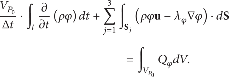
\frac{V_{P_{0}}}{Δ t} \cdot \int_{t} \frac{\partial}{\partial t} (ρ ϕ) d t + \sum_{j = 1}^{3} \int_{S_{j}} (ρ ϕ u - λ_{ϕ} \nabla ϕ) \cdot d S = \int_{V_{P_{0}}} Q_{ϕ} d V .

(21)

In comparison to the steady solver, the temporal term is not zero, and the first-order upwind difference scheme is adopted to discretize the term as follows:

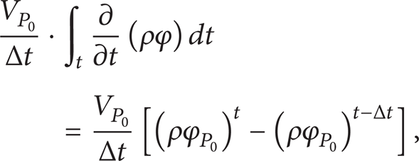
\frac{V_{P_{0}}}{Δ t} \cdot \int_{t} \frac{\partial}{\partial t} (ρ ϕ) d t = \frac{V_{P_{0}}}{Δ t} [{(ρ ϕ_{P_{0}})}^{t} - {(ρ ϕ_{P_{0}})}^{t - Δ t}],

(22)

where the superscript t – Δt denotes the previous time step.

The discretization of the convective flux, diffusion flux, source term, and pressure correction equation is the same as that for the steady solver above. The inlet in unsteady solver is set as the velocity boundary which changes with time. In each time step, the convergence conditions are the local and whole conservation of mass.

3.1.2. Unsteady Solver for Non-Newtonian Fluid

Similar to the introduction of the non-Newtonian fluid constitutive model in steady algorithm, the apparent viscosity μ_C calculated by the previous velocity field is used instead of Newtonian viscosity in simulation.

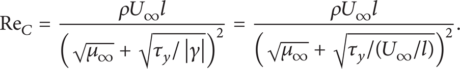
In unsteady non-Newtonian fluid flow, the generalized Reynolds number Re_C is related to the yield stress τ_y and defined by (23), which can better represent the non-Newtonian characteristics. When the yield stress τ_y is zero, (23) yields the same definition as that of Newtonian fluid flow:

R e_{C} = \frac{ρ U_{\infty} l}{{(\sqrt{μ_{\infty}} + \sqrt{τ_{y} / | γ |})}^{2}} = \frac{ρ U_{\infty} l}{{(\sqrt{μ_{\infty}} + \sqrt{τ_{y} / (U_{\infty} / l)})}^{2}} .

(23)

3.2. Validation of the Unsteady Solver

The lid-driven polar cavity flow used for the validation of the unsteady SIMPLE solver is shown schematically in Figure 7(a). The computation domain is discretized by 7502 triangle cells after grid independence test as shown in Figure 7(b). Initially, the flow is rest and the lid will rotate with circumferential velocity at t = 0. The Reynolds number Re based on the lid velocity and the depth of the cavity is 350. The normalized time t for the polar cavity flow is also based on the lid velocity and the depth of the polar. The time-step size Δt is 0.05. The measured velocity profiles can be found in the experiment by Fuchs and Tillmark [40].

Figure 7:

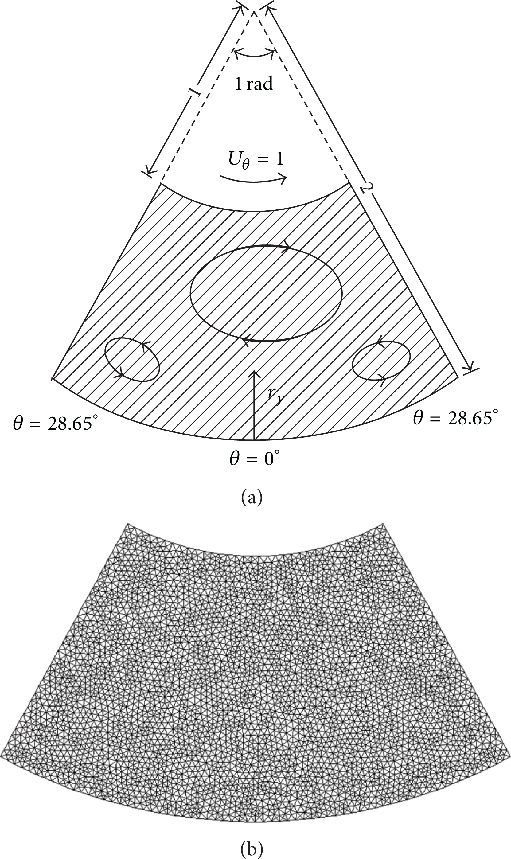
Lid-driven polar cavity flow staring from rest. (a) Schematic diagram [40]; (b) triangulation grid system.

The steady velocity profiles in θ = 0° section are compared with the simulation by Kim and Benson [41] and the measured results of Fuchs and Tillmark [40] in Figure 8, which shows that the results calculated using the present solver are in agreement with the experiment. The evolution of circumferential velocity U_θ at (r_y, θ) = (0.246, 0.0) is shown in Figure 9, comparing with the simulation results by Kim and Benson [41]. It is shown that the tendency of U_θ remains the same as the simulation results [41], and the convergent value is more identical with the steady experiment as shown by the dash line than that of Kim and Benson [41].

Figure 8:

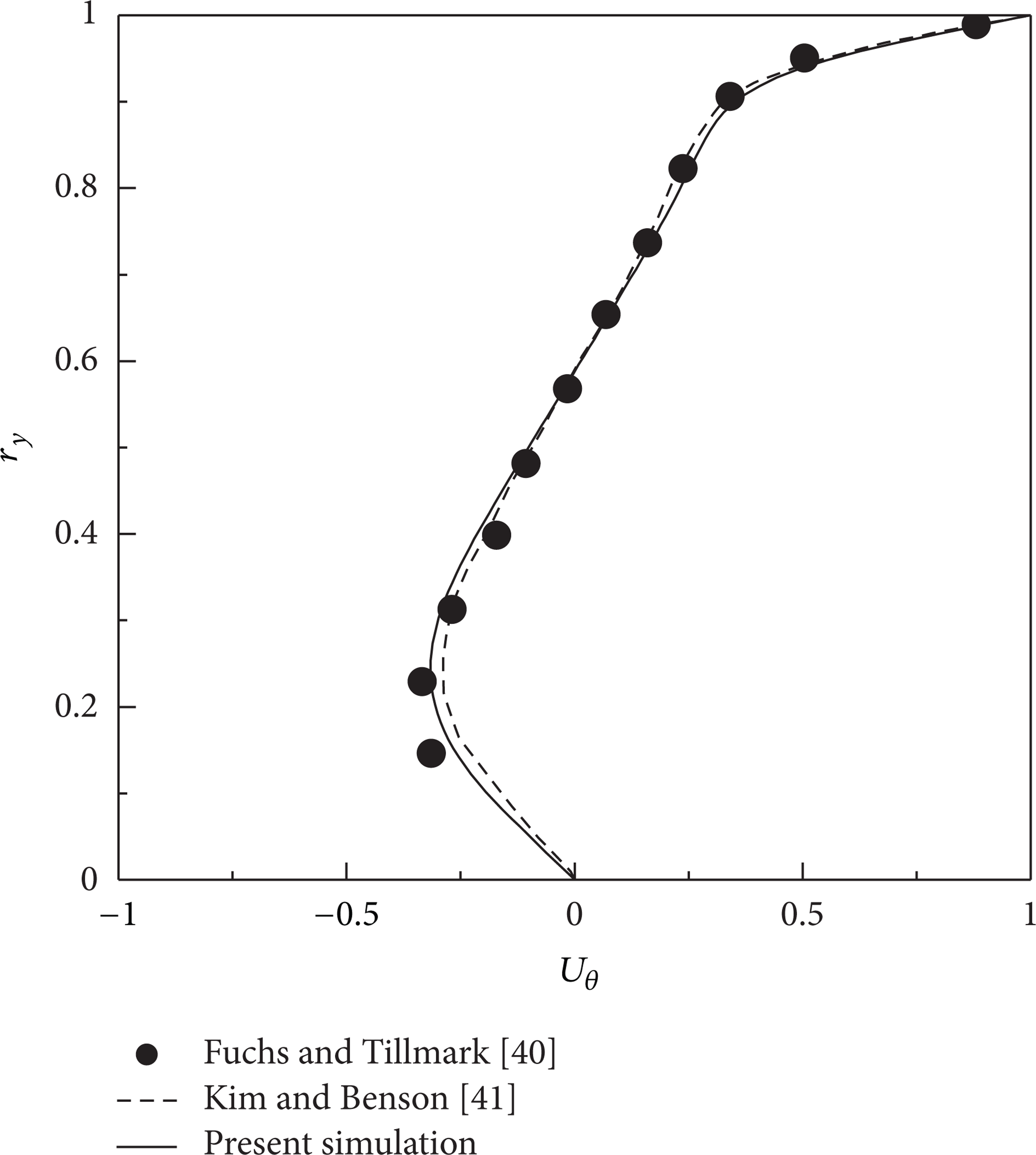
U_θ-velocity profiles in θ = 0° section.

Figure 9:

Evolution of U_θ at (r_y, θ) = (0.246, 0.0).

4. Blood Flow in Carotid Artery Bifurcation

Using the proposed unsteady SIMPLE solver, the blood flow in carotid artery bifurcation is simulated. The differences of blood flow under normotension and hypertension conditions are investigated in carotid artery bifurcation. In the section, we only give a prediction for atherosclerosis formation under hypertension using the theory that the enhancement of endothelial permeability and of lipid deposition preferentially occurs at low mean shear stress regions in the arteries [42, 43].

The carotid artery bifurcation is known as a site of atherosclerosis formation and is presumably influenced by the hemodynamics. Carotid atherosclerosis will lead to the formation of plaques in the carotid artery wall and insufficient brain supply, and atherosclerosis in serious can cause stroke, cerebral infarction, and even death. Clinical studies indicate that the hypertensive patients (hypertension stage I) are at higher risk of atherosclerosis formation than normotensive persons [44]. From the hemodynamics in the present study, we investigate the invasive sites and the mechanism of vulnerable sites of hypertensive patients.

For the simulation's convenience, the carotid artery bifurcation is simplified into Y-type bifurcation model, as shown in Figure 10. In the model, the diameter of the internal carotid d₁ = 0.71d₀ (d₀ is the diameter of common carotid) and the diameter of the external carotid d₂ = 0.568d₀. The bifurcation angle α is set as 50° [45] and the flow rate ratio between the internal and the external carotids is 0.7: 0.3 [45 –47]. The generalized Reynolds number in the inlet of common carotid is the same in the simulation. The physiologically realistic pulsatile wave form is shown in Figure 11, which is similar to the curve used in Berger and Jou [48] and the period of pulsatility is 1.0 second. As shown in the figure, the pulsatile wave of the hypertensive patients is remarkably different from that of the normal persons [49], and the diameter of the common carotid is also different. The diameter of the common carotid and the blood properties [50] of normal persons and hypertensive patients are shown in Table 1. The iteration is carried out for three pulses to ensure the stability of the results.

Table 1:

Diameter of the common carotid and blood parameters [50].

	d₀ (m)	τ_y (Pa)	μ_C (Pa · s)

Normal	0.0065	0.00877	0.00283
Hypertension	0.0074	0.01004	0.00363

Figure 10:

Carotid artery bifurcation model.

Figure 11:

Flow rate cure in the common carotid.

In the carotid artery bifurcation, the walls S1, S2, S3, and S4 are the vulnerable sites of atherosclerosis, and the internal carotid is more invasive. So the results are presented here for six points as shown in Figure 10 within a pulse period. For the point S4_5d₁, it means that the point is in the wall S4 and is 5d₁ from the bifurcation.

4.1. Model Validation and Grid Independence Test

To validate the present algorithm, a pulsatile blood flow in the common carotid under normal case is calculated. Figure 12 shows the velocity profile fully developed in the common carotid at t = 0.1 s, with the corresponding numerical result of Perktold et al. [51]. The present results are in good agreement with those numerical data. Four grids (7000, 10000, 20000, and 30000) are used to test the grid independence. It is shown that the profiles get overlapped one with another when the cell number is increased to 20000. Thus the mesh with 20000 cells is used below for the simulation of carotid bifurcation blood flow.

Figure 12:

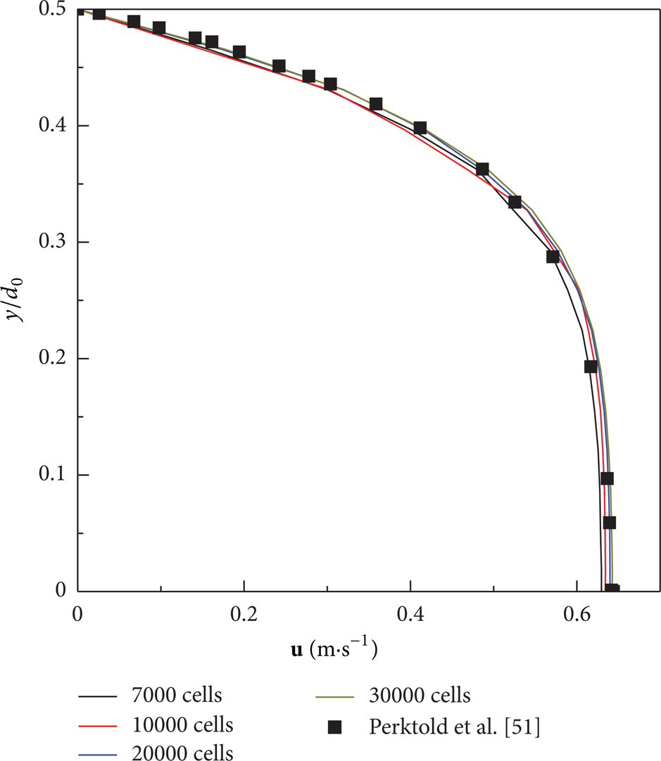
Fully developed velocity profiles in the common carotid at t = 0.1 s.

4.2. Results

The velocity vectors projections in carotid bifurcation at t₁ = 0.1 s and t₃ = 0.8 s are shown in Figure 13. As illustrated in the figure, the velocity of hypertensive patients is obviously higher than that of the normal persons. Especially at t₁ in Figure 13(a), the velocity in the internal carotid is 16.7%~21.05% higher than that of the normal persons and 15.38%~18.75% higher in the external carotid. The unusual higher blood velocity could have a harmful influence on the vascular wall cells of internal carotid and external carotid. Within a pulse period, negative axial velocity is also observed at the wall S1 one diameters downstream from the bifurcation, especially in hypertension case. The original living environmental of the endothelial cells in the internal and external carotids has been changed in hypertension case, and the endothelial cells need to bear bigger flow shock from the common carotid. So the larger flow shock from the common carotid flow cannot be ignored for hypertensive patients.

Figure 13:

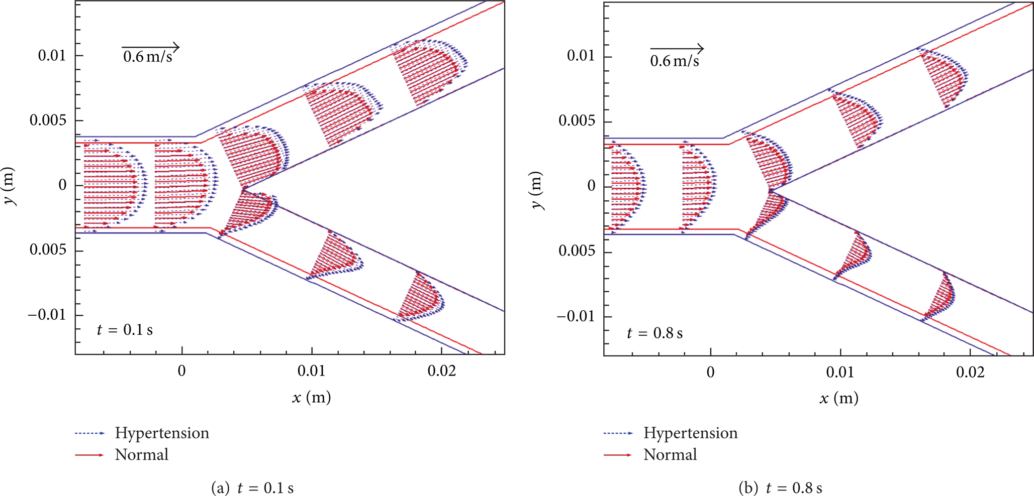
Velocity vectors projection in carotid bifurcation at different time: (a) t = 0.1 s, (b) t = 0.8 s.

Figure 14 presents the largest backflow regions that are, respectively, near the wall S1 and the wall S2, at t = 0.22 s. In the figure, the red regions are the backflow regions for the normal persons, while the blue hollow regions are the backflow regions for the hypertension patients. Ld_S1 is the largest back flow length in the external carotid for normal persons and Ld1_S2 is the largest back flow length in in the internal carotid for hypertension patients. As shown in the figure, for the hypertension patients, the largest backflow regions are much larger than those of the normal persons due to the high viscosity. Under present condition, the largest back flow length in the internal carotid is 78.5% longer than that for normal persons and 48.9% longer in the external carotid. For the hypertension patients, the larger area of the back flow is an important reason of the plaques formation in the wall S1 and the wall S2.

Figure 14:

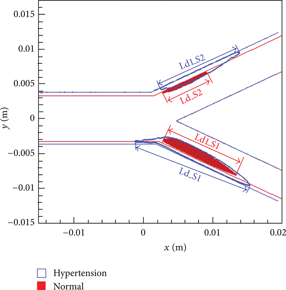
Backflow regions in carotid bifurcation at t = 0.22 s.

The time-WSS curves at the three points in the wall S2 are plotted in Figure 15. As evident in the figure, due to the backflow, the WSS peaks for the three points are obviously higher than that of the normal persons. With increasing the distance from the bifurcation, the reversed flow disappears, so WSS is higher gradually. WSS at the diastolic phase is 20%~87.1% lower than that of the normal persons, especially as shown in Figure 15(a). For three different points, the changing of time-WSS is also more than that of the normal persons. Thereby, for the hypertensive patients in the wall S2, the vessel wall is more invasive, and the plaques occur more easily.

Figure 15:

Distribution of the time-WSS in the wall S2 at different points: (a) S2_1d₁; (b) S2_2d₁; (c) S2_5d₁.

Figure 16 presents the distribution of the time-WSS at the three different points in the wall S4. As shown in the figure, due to the shock from the common carotid flow, WSS for the hypertensive patients is higher than that of the normal persons especially near the bifurcation, but with increasing the distance from the bifurcation and reducing the shock, the differences are lessened gradually. For point S4_5d₁ downstream the bifurcation, WSS at the diastolic phase is 3.7%~5.5% lower than that of the normal persons, as shown in Figure 16(c). Thereby, for the hypertensive patients in the wall S4, the possibility of atherosclerosis formation is increased especially downstream the bifurcation.

Figure 16:

Distribution of the time-WSS in the wall S4 at different points: (a) S4_1d₁; (b) S4_2d₁; (c) S4_5d₁.

The calculation shows that for the hypertensive patients, the possibility of the genesis and development of atherosclerosis is increased because of the increase in the incoming flow shock and backflow area in the wall S1 and S2 near the bifurcation, as well as the lower WSS distribution in the wall S3 and S4 downstream the bifurcation.

5. Conclusion

Taking into account the non-Newtonian and the pulsatile properties of the blood flow, we presented an unsteady solver for Casson fluid flow on unstructured collocated grid. The strong adaptability of unstructured grid to complex flow region can be used for the exact solution of blood flow in complex region in present solver. In the solver, the temporal term was discretized by first-order upwind difference scheme, which makes the solving process absolutely stable, low computational complexity, and small data storage. The Casson viscosity took the value calculated from the flow field of previous iteration in order to avoid the complexity caused by the complicated viscosity expression as a function of shear strain rate. In the present solver, Casson model can be used for the studies of blood rheology in the blood flow, which has not been implemented in commercial CFD software Fluent. The solving algorithm for Casson fluid can be used for all non-Newtonian fluids which can be described with τ = μ(|γ|)γ. The simulations of the lid-driven flow in polar cavity and the non-Newtonian fluid flow through a sudden expansion showed the validation of the unsteady solver and the feasibility of treatment of the shear stress and viscosity in non-Newtonian fluid flow, respectively. The calculation of blood flow in T-type bifurcation showed the necessity of using Casson model in simulation of blood flow.

Using the proposed algorithm, the blood flow of the hypertensive patients in the carotid artery bifurcation was simulated. For the hypertensive patients, the incoming velocity was 16.7%~21.05% higher in the internal carotid than that of the normal persons and 15.38%~18.75% higher in the external carotid. The largest back flow length was 78.5% longer in the internal carotid than that for normal persons and 48.9% longer in the external carotid. At the diastolic phase, WSS was 20%~87.1% lower in outer vascular wall near the bifurcation than that of the normal persons and 3.7%~5.5% lower in inner vascular wall downstream the bifurcation. The results showed that for the hypertensive patients, the most vulnerable sites were the outer vascular wall near the bifurcation and the inner vascular wall downstream the bifurcation. The reasons were mainly the lower WSS distribution and the increase in incoming flow shock and backflow area of the hypertensive patients.

Footnotes

Nomenclature

Greek Symbols

Acknowledgments

The support of the following projects is gratefully acknowledged: National Natural Science Foundation of China (no. 51176152), the Specialized Research Fund for the Doctoral Program of Higher Education (no. 20120201110070), the International Science & Technology Cooperation Plan of Shaanxi Province (no. 2013KW30-05), and Fundamental Research Funds for the Central Universities (xjj2012115). The authors would also like to acknowledge Professor Yu Bo from China University of Petroleum for technical support.

References

Ballyk

P. D.

Steinman

D. A.

, and Ethier

C. R.

, “Simulation of non-newtonial blood flow in an end-to-side anastomosis,” Biorheology, vol. 31, no. 5, pp. 565–586, 1994.

Taylor

C. A.

Hughes

T. J. R.

, and Zarins

C. K.

, “Finite element modeling of blood flow in arteries,” Computer Methods in Applied Mechanics and Engineering, vol. 158, no. 1–2, pp. 155–196, 1998.

Moore

and David

, “A model of autoregulated blood flow in the cerebral vasculature,” Proceedings of the Institution of Mechanical Engineers H, vol. 222, no. 4, pp. 513–530, 2008.

Chakravarty

and Sen

, “A mathematical model of blood flow in a catheterized artery with a stenosis,” Journal of Mechanics in Medicine and Biology, vol. 9, no. 3, pp. 377–410, 2009.

Deplano

Bailly

, and Bertrand

, “Influence of blood shear-thinning behaviour on flow dynamics in abdominal aortic aneurysm in vitro compliant model,” Computer Methods in Biomechanics and Biomedical Engineering, vol. 15, supplement 1, pp. 49–52, 2012.

Cho

Y. I.

and Kensey

K. R.

, “Effects of the non-Newtonian viscosity of blood on flows in a diseased arterial vessel. Part 1: steady flows,” Biorheology, vol. 28, no. 3–4, pp. 241–262, 1991.

Perktold

Resch

, and Florian

, “Pulsatile non-Newtonian flow characteristics in a three-dimensional human carotid bifurcation model,” Journal of Biomechanical Engineering, vol. 113, no. 4, pp. 464–475, 1991.

Fan

Jiang

Zou

Chen

, and Deng

, “Numerical simulation of pulsatile non-Newtonian flow in the carotid artery bifurcation,” Acta Mechanica Sinica, vol. 25, no. 2, pp. 249–255, 2009.

Rodkiewicz

C. M.

Sinha

, and Kennedy

J. S.

, “On the application of a constitutive equation for whole human blood,” Journal of Biomechanical Engineering, vol. 112, no. 2, pp. 198–206, 1990.

10.

Gijsen

F. J. H.

Van De Vosse

F. N.

, and Janssen

J. D.

, “The influence of the non-Newtonian properties of blood on the flow in large arteries: steady flow in a carotid bifurcation model,” Journal of Biomechanics, vol. 32, no. 6, pp. 601–608, 1999.

11.

Misra

J. C.

and Shit

G. C.

, “Role of slip velocity in blood flow through stenosed arteries: a non-Newtonian model,” Journal of Mechanics in Medicine and Biology, vol. 7, no. 3, pp. 337–353, 2007.

12.

Neofytou

and Drikakis

, “Non-Newtonian flow instability in a channelwith a sudden expansion,” Journal of Non-Newtonian Fluid Mechanics, vol. 111, no. 2–3, pp. 127–150, 2003.

13.

González

H. A.

and Moraga

N. O.

, “On predicting unsteady non-Newtonian blood flow,” Applied Mathematics and Computation, vol. 170, no. 2, pp. 909–923, 2005.

14.

Neofytou

and Tsangaris

, “Flow effects of blood constitutive equations in 3D models of vascular anomalies,” International Journal for Numerical Methods in Fluids, vol. 51, no. 5, pp. 489–510, 2006.

15.

Shah

S. R.

, “Study of modified Casson's fluid model in modeled normal and stenotic capillary-tissue diffusion phenomena,” International Journal of Computational Engineering & Management, vol. 11, pp. 51–57, 2011.

16.

Merrill

E. W.

Benis

A. M.

Gilliland

E. R.

Sherwood

T. K.

, and Salzman

E. W.

, “Pressure-flow relations of human blood in hollow fibers at low flow rates,” Journal of Applied Physiology, vol. 20, no. 5, pp. 954–967, 1965.

17.

Scott Blair

G. W.

, “The success of Casson's equation,” Rheologica Acta, vol. 5, no. 3, pp. 184–187, 1966.

18.

Walawender

W. P.

Chen

T. Y.

, and Cala

D. F.

, “An approximate casson fluid model for tube flow of blood,” Biorheology, vol. 12, no. 2, pp. 111–119, 1975.

19.

Cebral

and Lohner

, “Automatic grid generation for anatomically accurate computational hemodynamics calculations,” in Proceedings of International Conference on Mechanics in Medicine and Biology (ICMMB '11), Maui, Hawaii, USA, 2000.

20.

Tao

W. Q.

, Modern Progress of Computational Heat Transfer, Science Press, Beijing, China, 1st edition, 2000.

21.

Chen

and Lu

X. Y.

, “Numerical investigation of the non-Newtonian blood flow in a bifurcation model with a non-planar branch,” Journal of Biomechanics, vol. 37, no. 12, pp. 1899–1911, 2004.

22.

Chen

and Lu

X. Y.

, “Numerical investigation of the non-Newtonian pulsatile blood flow in a bifurcation model with a non-planar branch,” Journal of Biomechanics, vol. 39, no. 5, pp. 818–832, 2006.

23.

Perktold

Peter

R. O.

Resch

, and Langs

, “Pulsatile non-Newtonian blood flow in three-dimensional carotid bifurcation models: a numerical study of flow phenomena under different bifurcation angles,” Journal of Biomedical Engineering, vol. 13, no. 6, pp. 507–515, 1991.

24.

Perktold

Resch

, and Peter

R. O.

, “Three-dimensional numerical analysis of pulsatile flow and wall shear stress in the carotid artery bifucation,” Journal of Biomechanics, vol. 24, no. 6, pp. 409–420, 1991.

25.

D. N.

and Giddens

D. P.

, “Pulsatile flow in a model carotid bifurcation,” Arteriosclerosis, vol. 3, no. 1, pp. 31–39, 1983.

26.

Jou

L. D.

and Berger

S. A.

, “Numerical simulation of the flow in the carotid bifurcation,” Theoretical and Computational Fluid Dynamics, vol. 10, no. 1–4, pp. 239–248, 1998.

27.

Lee

M. Y.

C. M.

K. H.

, “Association between wall shear stress and carotid atherosclerosis in patients with never treated essential hypertension,” American Journal of Hypertension, vol. 22, no. 7, pp. 705–710, 2009.

28.

Gleason

R. L.

and Humphrey

J. D.

, “A mixture model of arterial growth and remodeling in hypertension: altered muscle tone and tissue turnover,” Journal of Vascular Research, vol. 41, no. 4, pp. 352–363, 2004.

29.

Vasava

Jalali

Dabagh

, and Kolari

P. J.

, “Finite element modelling of pulsatile blood flow in idealized model of human aortic arch: study of hypotension and hypertension,” Computational and Mathematical Methods in Medicine, vol. 2012, Article ID 861837, 14 pages, 2012.

30.

Tang

B. T.

Pickard

S. S.

Chan

F. P.

Tsao

P. S.

Taylor

C. A.

, and Feinstein

J. A.

, “Wall shear stress is decreased in the pulmonary arteries of patients with pulmonary arterial hypertension: an image-based, computational fluid dynamics study,” Pulmonary Circulation, vol. 2, no. 4, pp. 470–476, 2012.

31.

Chen

and Guo

L. J.

, “Quick generation of unstructured grid,” Journal of Xi'an Jiao Tong University, vol. 34, no. 1, pp. 18–21, 2000.

32.

Tao

W. Q.

, Numerical Heat Transfer, Xi'an Jiao Tong University Press, Xi'an, China, 2nd edition, 2001.

33.

Wang

, and Tao

, “Study on general governing equations of computational heat transfer and fluid flow,” Communications in Computational Physics, vol. 12, no. 5, pp. 1482–1494, 2012.

34.

Rhie

C. M.

and Chow

W. L.

, “Numerical study of the turbulent flow past an airfoil with trailing edge separation,” AIAA Journal, vol. 21, no. 11, pp. 1525–1532, 1983.

35.

Scott Blair

G. W.

, “An equation for the flow of blood, plasma and serum through glass capillaries,” Nature, vol. 183, no. 4661, pp. 613–614, 1959.

36.

Papanastasiou

T. C.

, “Flows of materials with yield,” Journal of Rheology, vol. 31, no. 5, pp. 385–404, 1987.

37.

Pham

T. V.

and Mitsoulis

, “Entry and exit flows of Casson fluids,” Canadian Journal of Chemical Engineering, vol. 72, no. 6, pp. 1080–1084, 1994.

38.

Neofytou

, “Transition to asymmetry of generalised Newtonian fluid flows through a symmetric sudden expansion,” Journal of Non-Newtonian Fluid Mechanics, vol. 133, no. 2–3, pp. 132–140, 2006.

39.

Talukder

and Nerem

, “Flow characteristics in vascular graft models,” in Proceedings of the International Conference on Mechanics in Medicine and Biology, vol. 7, pp. 281–284, Verlag Gerhard Witzstrock, 1987.

40.

Fuchs

and Tillmark

, “Numerical and experimental-study of driven flow in a polar cavity,” International Journal for Numerical Methods in Fluids, vol. 5, no. 4, pp. 311–329, 1985.

41.

Kim

S. W.

and Benson

T. J.

, “Comparison of the SMAC, PISO and iterative time-advancing schemes for unsteady flows,” Computers and Fluids, vol. 21, no. 3, pp. 435–454, 1992.

42.

Yoshida

Wang

Yamane

, “Structural differences of arterial walls which are either vulnerable or resistant to atherosclerosis,” Acta Medica et Biologica, vol. 38, supplement 1, pp. 1–19, 1990.

43.

Okano

and Yoshida

, “Influence of shear stress on endothelial cell shapes and junction complexes at flow dividers of aortic bifurcations in cholesterol-fed rabbits,” Frontiers of Medical and Biological Engineering, vol. 5, no. 2, pp. 95–120, 1993.

44.

J. J.

Baek

, and Humphrey

J. D.

, “Stress-strain behavior of the passive basilar artery in normotension and hypertension,” Journal of Biomechanics, vol. 40, no. 11, pp. 2559–2563, 2007.

45.

P. P.

X. M.

, and Ku

D. N.

, “Convective mass transfer at the carotid bifurcation,” Journal of Biomechanics, vol. 30, no. 6, pp. 565–571, 1997.

46.

Ding

Z. R.

Wang

K. Q.

, and Cong

X. S.

, “Study on the flow separation in human carotid bifurcation,” Journal of Medical Biomechanics, vol. 17, pp. 28–32, 2002.

47.

D. N.

Giddens

D. P.

Zarins

C. K.

, and Glagov

, “Pulsatile flow and atherosclerosis in the human carotid bifurcation. Positive correlation between plaque location and low and oscillating shear stress,” Arteriosclerosis, vol. 5, no. 3, pp. 293–302, 1985.

48.

Berger

S. A.

and Jou

L.-D.

, “Flows in stenotic vessels,” Annual Review of Fluid Mechanics, vol. 32, pp. 347–382, 2000.

49.

Hajdu

M. A.

and Baumbach

G. L.

, “Mechanics of large and small cerebral arteries in chronic hypertension,” American Journal of Physiology, vol. 266, no. 3, pp. H1027–H1033, 1994.

50.

Mao

Chou

Z. J.

Wang

J. Y.

, “Hemorheology examination parameters and Casson equation index and common geriatric disease,” Chinese Journal of Hemorheology, vol. 12, no. 2, pp. 114–117, 2002.

51.

Perktold

Resch

, and Florian

, “Pulsatile non-Newtonian flow characteristics in a three-dimensional human carotid bifurcation model,” Journal of Biomechanical Engineering, vol. 113, no. 4, pp. 464–475, 1991.

Unsteady Non-Newtonian Solver on Unstructured Grid for the Simulation of Blood Flow

Abstract

1. Introduction

2. Steady Solver on Unstructured Grid

2.1. Steady Solver for Newtonian Fluid

2.1.1. Solution of Flow Field

2.1.2. Correction of Pressure

2.1.3. Discretization of Boundary Condition and Convergence Conditions

2.2. Steady Solver for Non-Newtonian Fluid

2.3. Validation of the Non-Newtonian Model in Steady Solver

2.3.1. Non-Newtonian Fluid Flow through a Sudden Expansion

2.3.2. Steady Blood Flow in T-Type Bifurcation

3. Unsteady Solver on Unstructured Grid

3.1. Unsteady Algorithm

3.1.1. Discretization of the Governing Equation

3.1.2. Unsteady Solver for Non-Newtonian Fluid

3.2. Validation of the Unsteady Solver

4. Blood Flow in Carotid Artery Bifurcation

4.1. Model Validation and Grid Independence Test

4.2. Results

5. Conclusion

Footnotes

Nomenclature

Greek Symbols

Acknowledgments

References