A Modified k -ε Model for Computation of Flows with Large Streamline Curvature

Abstract

This paper presents an improved method for inclusion of system rotation and streamline curvature effects into existing two-equation eddy-viscosity turbulence models. A new formulation for calculation of the turbulence viscosity coefficient, which is implemented into the traditional k-ε model with a two-layer near-wall treatment in a commercial computational fluid dynamics solver, is proposed. In contrast to precious model, the modified rotation rate which appears in the formulation for turbulent viscosity coefficient is herein expressed exactly and universally. Thus, it provides an effective alternative for turbulence modeling.

1. Introduction

The use of computational fluid dynamics (CFD) for prediction of complex flows has brought about substantial improvements in analysis for the design of industrial products. For high Reynolds number flow, one critical aspect of the CFD model is the turbulence model used. Among existing technologies, direct numerical simulation (DNS) and large eddy simulation (LES) are the most theoretically complete modeling approaches used to predict turbulent flows. However, these methods require significant computational resources, including both memory and processing power, and current estimates by Spalart [1] suggest that it will be several years, if not decades, before these become viable alternatives for analysis of large-scale, complex flow fields for industrial design purposes. Reynolds-averaged Navier-Stokes methods (RANS) are therefore commonly used in practice as a compromise between computational efficiency and reasonable accuracy. Among RANS modeling methods, two-equation eddy-viscosity models (the standard k-ε model) are the most popular and have been shown to provide the capability for engineering-level predictions. However, these models suffer a reduction in accuracy as the physics encountered in particular flow fields become more complex. For example, in many industrial designs, including turbomachinery applications, the flow is subjected to streamline curvature and/or reference frame rotation [2, 3], which challenges the accuracy of existing two-equation eddy-viscosity models.

In an effort to more accurately resolve these complex flow physics, researchers have recently sought to develop models that more accurately predict the effects of curvature and rotation on turbulent flow. In theory, differential Reynolds stress models are the most accurate RANS models but are also the most complicated, since they solve a transport equation for each of the six independent turbulent stress components. One advantage to these models is that sensitivity to streamline curvature and reference frame rotation is naturally addressed. However, this approach is still not commonly used in industrial applications due to excessive computational cost and computational stiffness. On the other hand, the eddy-viscosity models widely used in engineering applications follow the Boussinesq assumption, which relates the turbulent stress components to the mean strain rate via a turbulent viscosity and characterize the turbulence only through scalar transport variables such as k, ε, ω, or ν _T . The effect of rotation and curvature on turbulence dynamics is due to Reynolds stress anisotropy, which is not directly included in most scalar eddy-viscosity models. Due to the lack of any direct sensitivity of these to streamline curvature and reference frame rotation, most popular eddy-viscosity models like the k-ε model and k-ω model may lead to large errors in the prediction of complex flow situations such as those encountered in turbomachinery applications.

Several researchers have attempted to incorporate physically realistic rotation and curvature sensitivity into scalar eddy-viscosity models. Initially these were based on ad hoc modifications to the model formulations, and in many cases did not satisfy mathematical invariance principles, a necessary condition for general-purpose modeling methods. More recently, methods have been developed which attempt to incorporate the advantages of both eddy-viscosity models (simplicity, computational efficiency) and Reynolds stress models (physically correct response to curvature and rotation). For example, Spalart and Shur [4] improved the original S-A model through the modification of production terms, while Pettersson Reif et al. [5] proposed a nonlinear eddy-viscosity turbulence model which responds correctly to both stabilizing and destabilizing curvature.

Alternatively, York et al. [6] proposed a simple modified form of the turbulent viscosity coefficient (C_μ) to incorporate rotation and curvature effects, and the resulting k-ε model was validated by typical flow cases such as rotating channel flow, U-bend flow, and internally cooled turbine airfoil conjugate heat transfer. The model satisfies realizability and invariance principles and was presented as a simple “plug-in” for use with existing two-equation turbulence models. The effect of curvature and rotation is included in the turbulent viscosity coefficient via the effective rotation rate magnitude term, which was approximated by York et al. [6] based on the assumption that the local flow conditions correspond to two-dimensional, simple shear flow in a frame rotating with the flow. For the test cases considered, the model was found to make a significant improvement in two-dimensional flow problems. However, industrial flows are often very complex, and the idealization of plane shear flow may be far from the actuality of the local flow conditions. For these cases it is expected that the simple assumption may lose its effectiveness. In an attempt to improve the performance of the model, and based on the work of Wallin and Johansson [7], an exact calculation of the effective rotation rate magnitude is adopted in this paper, which is intended to make the model more universal, while retaining the advantage of providing a simple “plug-in” solution for capturing rotation and curvature effects in two-equation eddy viscosity models.

The new eddy-viscosity coefficient expression was implemented into a two-layer k-ε model in the same manner as that in [6]. In the present study, the model was tested for two representative flow problems. First, simple U-bend flow was tested to compare the differences between the current model, and the original model presented by York et al. Flow was then calculated through a 90° bend model to assess the performance of the models for a simple case that includes three-dimensional effects and strong streamline curvature. All the numerical simulations have been compared with available experimental data available in terms of both mean flow and turbulence quantities.

2. Model Development

The anisotropy tensor (b _ij ) for incompressible flow can be expressed in terms of turbulent kinetic energy (k) and the Reynolds stress tensor as

$b_{ij}=\frac{\stackrel{——}{u_i{u}_j}}{k}-\frac{\mathrm{2}}{\mathrm{3}}{\delta }_{ij},$

(1)

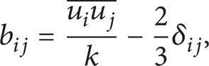
where δ _ij is the Kronecker delta. The anisotropy tensor contains relevant information on the turbulence structure and must be evaluated as a function of available variables in the simulation. For linear eddy-viscosity models, the anisotropy tensor is directly related to the turbulent viscosity as follows:

$b_{ij}=-\frac{\mathrm{2}{\nu }_T{s}_{ij}}{k}.$

(2)

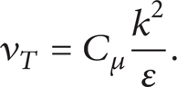
Here, ν _T is the turbulent viscosity. Gatski and Speziale [8] proposed an explicit functional form for the anisotropy tensor, based on the weak equilibrium hypothesis, to develop an algebraic Reynolds stress model. Starting with the differential Reynolds stress transport equations, neglecting convective and transport terms, and under the assumption of weak equilibrium, it was shown that

$b_{ij}=\frac{\left(\left(\mathrm{4}/\mathrm{3}\right)-C_{\mathrm{2}}\right)}{\left(C_{\mathrm{3}}-\mathrm{2}\right)}\frac{\mathrm{6}}{\mathrm{3}-\mathrm{2}{\eta }^{\mathrm{2}}+\mathrm{6}{\zeta }^{\mathrm{2}}}\times [S_{ij}^{*}+(\phantom{\left(S_{ik}^{*}{S}_{kj}^{*}-\frac{\mathrm{1}}{\mathrm{3}}{S}_{kl}^{*}{S}_{kl}^{*}{\delta }_{ij}\right)}{S}_{ik}^{*}{W}_{ik}^{*}+S_{jk}^{*}{W}_{ki}^{*}\hspace{0.17em}-\mathrm{2}\left(S_{ik}^{*}{S}_{kj}^{*}-\frac{\mathrm{1}}{\mathrm{3}}{S}_{kl}^{*}{S}_{kl}^{*}{\delta }_{ij}\right))].$

(3)

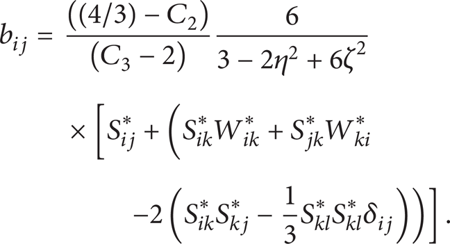
The terms in (3) are constructions of the mean flow quantities as well as the turbulence transport variables. For a k-ε based model:

${\eta }^{\mathrm{2}}=S_{ij}^{*}{S}_{ij}^{*},$

(4)

${\zeta }^{\mathrm{2}}=W_{ij}^{*}{W}_{ij}^{*},$

(5)

$S_{ij}^{*}=\frac{\mathrm{1}}{\mathrm{2}}g\frac{k}{\epsilon }\left(\mathrm{2}-C_{\mathrm{3}}\right)S_{ij},$

(6)

$W_{ij}^{*}=\frac{\mathrm{1}}{\mathrm{2}}g\frac{k}{\epsilon }\left(\mathrm{2}-C_{\mathrm{4}}\right)W_{ij},$

(7)

$W_{ij}={\mathrm{\Omega }}_{ij}^{\prime }+\frac{C_{\mathrm{4}}-\mathrm{4}}{C_{\mathrm{4}}-\mathrm{2}}{e}_{mji}{\omega }_m,$

(8)

$g={\left(\frac{\mathrm{1}}{\mathrm{2}}{C}_{\mathrm{1}}+\frac{P^k}{\epsilon }-\mathrm{1}\right)}^{-\mathrm{1}}.$

(9)

Here S _ij denotes the mean rate-of-strain tensor, and ${\mathrm{\Omega }}_{ij}^{\prime }$ denotes the mean rotation rate tensor, both expressed in a reference frame rotating with angular velocity ω _m as follows:

$\begin{array}{c}{S}_{ij}^{}=\frac{\mathrm{1}}{\mathrm{2}}\left(\frac{\partial U_i}{\partial x_j}+\frac{\partial U_j}{\partial x_i}\right),\\ {\mathrm{\Omega }}_{ij}^{\prime }=\frac{\mathrm{1}}{\mathrm{2}}\left(\frac{\partial U_i}{\partial x_j}-\frac{\partial U_j}{\partial x_i}\right).\end{array}$

(10)

Model coefficients C₁–C₄ are defined in [8].

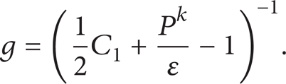
The above equations (3)–(9), along with the turbulent kinetic energy (k) represent a nonlinear expression for the Reynolds stress tensor in terms of available mean flow and turbulent statistical variables. In order to develop an improved linear eddy-viscosity model, York et al. [6] adopted the first (linear) term in (3) to develop a semi-implicit expression for the turbulent viscosity coefficient. The process is to linearize the anisotropy tensor with respect to the mean strain rate. Based on k-ε model, the turbulent viscosity ν _T in (2) is defined as

${\nu }_T=C_{\mu }\frac{k^{\mathrm{2}}}{∊}.$

(11)

The deduced expression of C_μ is

$C_{\mu }=\frac{K_{\mathrm{1}}+K_{\mathrm{2}}{C}_{\mu }{\left(Sk/∊\right)}^{\mathrm{2}}+K_{\mathrm{3}}{C}_{\mu }\left(Sk/∊\right)+K_{\mathrm{4}}{C}_{\mu }^{\mathrm{2}}{\left(Sk/∊\right)}^{\mathrm{3}}}{K_{\mathrm{5}}+K_{\mathrm{6}}{C}_{\mu }{\left(Sk/∊\right)}^{\mathrm{2}}+K_{\mathrm{7}}{C}_{\mu }^{\mathrm{2}}{\left(Sk/∊\right)}^{\mathrm{4}}+K_{\mathrm{8}}{\left(Wk/∊\right)}^{\mathrm{2}}}.$

(12)

To see the detailed derivation from (4) to (12), refer to the appendix of the paper by York et al. In the above, S is the strain rate magnitude, K₁–K₈ are model constants that can be expressed as algebraic functions of C₁–C₄, and ε is the turbulence dissipation rate.

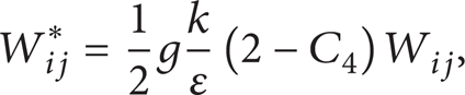
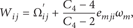
The effect of curvature and rotation is included through the term ω _m and enters into the eddy-viscosity expression via the effective rotation rate magnitude term W that appears in (12) as follows:

$W=\sqrt{\mathrm{2}{W}_{ij}{W}_{ij}}.$

(13)

Note that (8) can be alternatively expressed as follows:

$W_{ij}={\mathrm{\Omega }}_{ij}^{\prime }+e_{mji}{\omega }_m+\frac{-\mathrm{2}}{C_{\mathrm{4}}-\mathrm{2}}{e}_{mji}{\omega }_m,$

(14)

$W_{ij}={\mathrm{\Omega }}_{ij}+\frac{\mathrm{2}}{C_{\mathrm{4}}-\mathrm{2}}{\mathrm{\Omega }}_{ij}^r,$

(15)

where ${\mathrm{\Omega }}_{ij}={\mathrm{\Omega }}_{ij}^{\prime }+e_{mji}{\omega }_m$ is the absolute vorticity tensor, expressed in an inertial frame of reference, and ${\mathrm{\Omega }}_{ij}^r=-e_{mji}{\omega }_m$ is the coordinate system rotation rate tensor, also referred to as the vorticity modification tensor by Girimaji [9]. Although mathematically similar, the effect of a rotating reference frame modifies the vorticity uniformly everywhere in the flow field, whereas the influence due to curvature effects varies as a function of both time and space throughout the domain.

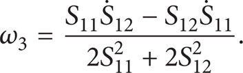
In order to ensure frame indifference and to include the effects of both system rotation and streamline curvature on the eddy viscosity, the term ω _m that appears in (14) is taken to be the local Lagrangian rotation rate of the principal axes of the mean strain rate tensor. This is similar to previous approaches taken in the literature [4, 10–12]. Therefore, in order to close the model, ω _m must be computed from the mean velocity field. In the present model formulation, we make use of the derivation by Wallin and Johansson [13] for ω _m , which was also adopted by Spalart and Shur [4] and Gatski and Jongen [10] for curvature-corrected versions of the S-A model and an algebraic Reynolds stress model, respectively as follows:

${\omega }_i=A_{ij}^{-\mathrm{1}}{S}_{pl}{\stackrel{.}{S}}_{lq}{e}_{pqj},$

(16)

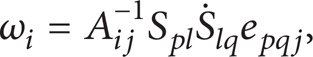
where ${\stackrel{.}{S}}_{ij}$ is the material derivative of the strain rate tensor and

$A_{ij}^{-\mathrm{1}}=\frac{\text{I}{\text{I}}_s^{\mathrm{2}}{\delta }_{ij}+\mathrm{12}\text{II}{\text{I}}_s{S}_{ij}+\mathrm{6}\text{I}{\text{I}}_s{S}_{ik}{S}_{kj}}{\mathrm{2}\text{I}{\text{I}}_s^{\mathrm{3}}-\mathrm{12}\text{II}{\text{I}}_s^{\mathrm{2}}}.$

(17)

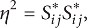
Here II _s and III _s are second and third invariants of the mean strain rate tensor. For two-dimensional mean flows, (16) reduces to

${\omega }_{\mathrm{3}}=\frac{S_{\mathrm{11}}{\stackrel{.}{S}}_{\mathrm{12}}-S_{\mathrm{12}}{\stackrel{.}{S}}_{\mathrm{11}}}{\mathrm{2}{S}_{\mathrm{11}}^{\mathrm{2}}+\mathrm{2}{S}_{\mathrm{12}}^{\mathrm{2}}}.$

(18)

Equation (16) represents the key difference between the model proposed here and the original linear eddy-viscosity model. As stated above, that previous model form utilized a simple approximation for the vorticity modification tensor and effective rotation rate magnitude (W). For purposes of comparison between the two model forms, the previous model terms are included here:

$\begin{array}{c}{\omega }_m=\mathrm{0.5}\left(S-\mathrm{\Omega }\right),\\ W=\left(\frac{\mathrm{4}-C_{\mathrm{4}}}{\mathrm{2}-C_{\mathrm{4}}}\right)\mathrm{\Omega }-\left(\frac{\mathrm{2}}{\mathrm{2}-C_{\mathrm{4}}}\right)S,\\ \mathrm{\Omega }=\sqrt{\mathrm{2}{\mathrm{\Omega }}_{ij}{\mathrm{\Omega }}_{ij}}.\end{array}$

(19)

The turbulent viscosity coefficient represented by (6), (12)–(14), (16), and (17) was implemented within a k-ε model for which the high Reynolds number form matched that of the standard implementation (Launder and Spalding [14]). All other details of the model, including model constants and two-layer near-wall treatment, are identical to those used in [6], and the reader is referred there for a complete description.

3. Numerical Details

The turbulent viscosity formulation outlined above was implemented into Fluent version 6.3.26 via user defined functions (UDF). For comparison, simulations of test cases were also conducted with the standard k-ε (denoted SKE) model and the simple modified model of York et al. [6] (denoted SKE-S). The new model is denoted as SKE-C. Simulations were run using the SIMPLEC pressure-correction solver with the QUICK convective scheme for all flow variables. Due to the incorporation of the second order derivative of velocity in the computation of the rotation rate term (16), the turbulent viscosity was under relaxed during the iterating process, and a value of 0.3 was found to be suitable to maintain stability in all of the current test cases. The criteria used to determine the convergence of the solutions was the same as that used in [6].

A grid sensitivity study was carried out for all cases, which was realized with the help of the solution-based grid adaption technology in Fluent. When the initial solution was obtained, the basic grid was refined, and the process repeated until the all relevant solution parameters were unchanging. The grids used for the results presented below were all deemed to be grid independent based on this approach. To illustrate the process in more detail, the approach for a typical example is illustrated in the following section.

For the two-dimensional case (U-bend flow), the computation was run on two processors of a Lenovo computer with 2.2 GHz and 2.0 GB RAM. The three-dimensional cases (90° bend) were run on 16 processors of a parallel computing cluster DeepComp 1800 with 8 CPUs × 1.9 GHz and 8 GB RAM. The SKE-C model took no more than 10 percent more computational time per iteration than the SKE and SKE-S models. The extra time can be attributed to the calculation of the second order velocity derivatives. The total number of iterations needed for convergence was approximately 50% more than the other two models, due most likely to the under relaxation of the turbulent viscosity.

4. Test Cases

To assess the performance of the new model, two test cases were performed, and results were compared with available experimental data. The chosen cases are representative of flows commonly encountered in industrial applications and include the following: (1) two-dimensional U-bend flow, which is intended primarily to check whether the new model has better performance than the original simple curvature-corrected model; (2) three-dimensional 90° bend flow which serves as a simple test to demonstrate the response of the models to more complex vortex flows. These cases were chosen based on the fact that they exhibit significant streamline curvature without the additional complications often encountered in industrial flows such as separation, unsteadiness, and transition. This allows a comparison between the turbulence models based solely on their ability to resolve rotation/curvature effects. It should also be pointed out that the test cases considered do not include flow in a rotating reference frame. It has been previously noted in a number of studies that frame rotation rate does not influence turbulent flow characteristics per se, since it merely defines the observational point of reference. Any flow field can be cast in either a rotating or inertial frame arbitrarily. Rather, it is the local flow rotation, as described by the Lagrangian rotation rate of the mean strain rate principal axes, which influences the turbulence structure. Therefore, as pointed out by Spalart and Shur [4], system rotation is exactly analogous with streamline curvature, hence only cases with obvious streamline curvature were investigated in this study.

5. U-Bend Flow

Two-dimensional U-bend flow is a canonical benchmark to validate the sensitivity of a turbulence model to streamline curvature. The simulation here follows the experimental geometry and conditions of [15]. The simulation domain is illustrated in Figure 1. The numerical details are the same as those in [6] except that the profile of turbulent kinetic energy at the inlet s/H = 0 (s denotes streamwise coordinate, h used in figures bellow denotes transverse coordinate, and H is the height of the bend) was prescribed, so that it matched the experiment precisely, which is shown in Figure 2.

Figure 1:

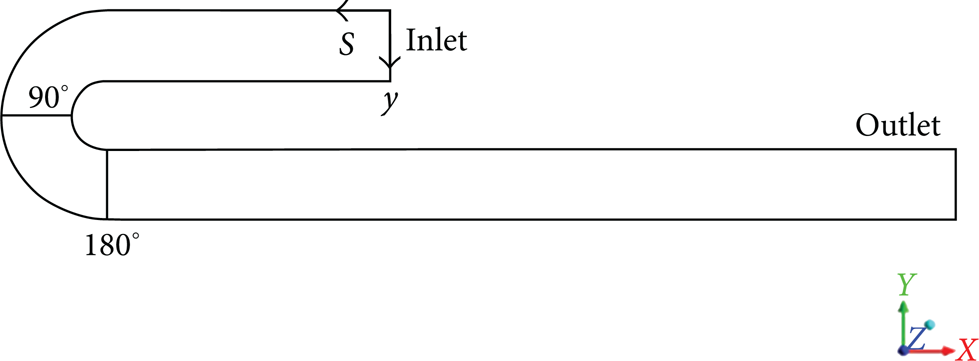
Two-dimensional U-bend geometry.

Figure 2:

Profile of the turbulent kinetic energy at the inlet compared with experimental data.

To get a solution independent of grid, three grid sets with different grid density (729 × 33, 1460 × 66, and 2200 × 100 in the streamwise and wall normal directions, resp.) were tested. Comparing the streamwise velocity normalized by the averaged velocity at the inlet, Figure 3 indicates that results calculated using each of the three grids are in good agreement with one another except in the region 0 < h/H < 0.1. An enlarged view of this zone shown on the right side of Figure 3 indicates that the middensity grid (1460 × 66) is sufficiently accurate for the present study, and the remaining results presented in this section were obtained on this grid.

Figure 3:

Profiles of normalized streamwise velocity at θ = 90° in the 2D U-bend, obtained using grids with three different refinement levels.

Figure 4 shows the flow development at the 90° bend section in terms of the streamwise velocity (u) and turbulent kinetic energy (k) profiles, each normalized by the average velocity U _m across the channel. Observing the velocity distribution, the acceleration on the convex side and the deceleration on the concave side are readily apparent. Although simulations with all three models show reduced velocity magnitude relative to the experimental data on the convex side, the result obtained from the new model (SKE-C) is the most accurate. Furthermore, it is known that the convex curvature has a stabilizing effect on the turbulence, while the concave curvature has a destabilizing effect. Observing the profiles of turbulent kinetic energy calculated by the different models, it is evident that the SKE model is completely insensitive to curvature effects, with a reverse distribution of k, while the SKE-S model and SKE-C model show better agreement with the experimental data. Between the two curvature-sensitized models, the results using the SKE-C model match the shape and magnitude of the turbulent kinetic energy quite well, especially near the inner wall, and overall show better performance than the SKE-S model.

Figure 4:

Profiles of normalized streamwise velocity and turbulent kinetic energy at θ = 90° in the 2D U-bend.

Figure 5 shows the profiles for k and u at θ = 180°, which corresponds to the exit of the U-bend region. Experimental data show that a separation bubble exists at this location near the inner side wall. Only the SKE-S and SKE-C capture the negative streamwise velocity indicative of reverse flow. These two models predict reduced turbulent viscosity values near the inner wall, which result in separation of the boundary layer due to the adverse pressure gradient, while the SKE model predicts elevated turbulence levels typical of nonrotating flow, and therefore fails to resolve the separation. From the profiles of k, it is apparent that the SKE-C model results are closest to measured data. The most significant difference between data and model results is found in the large peak of turbulent kinetic energy on the inner wall. York et al. [6] hypothesized that this peak is induced by the unsteady characteristics of the separated shear layer, and that RANS models in general are ill suited to accurately capture the phenomenon of shear layer instability and breakup.

Figure 5:

Profiles of normalized streamwise velocity and turbulent kinetic energy at θ = 180° in the 2D U-bend.

With regard to the size of the separation bubble, Figure 6 shows the streamlines predicted by all three of the models. It is clear that the bubble calculated by SKE-C is the largest but still smaller than that observed in the experiment. In contrast, the SKE-S model shows a smaller separation bubble, while the SKE model, as mentioned above, fails to capture any separation downstream of the bend.

Figure 6:

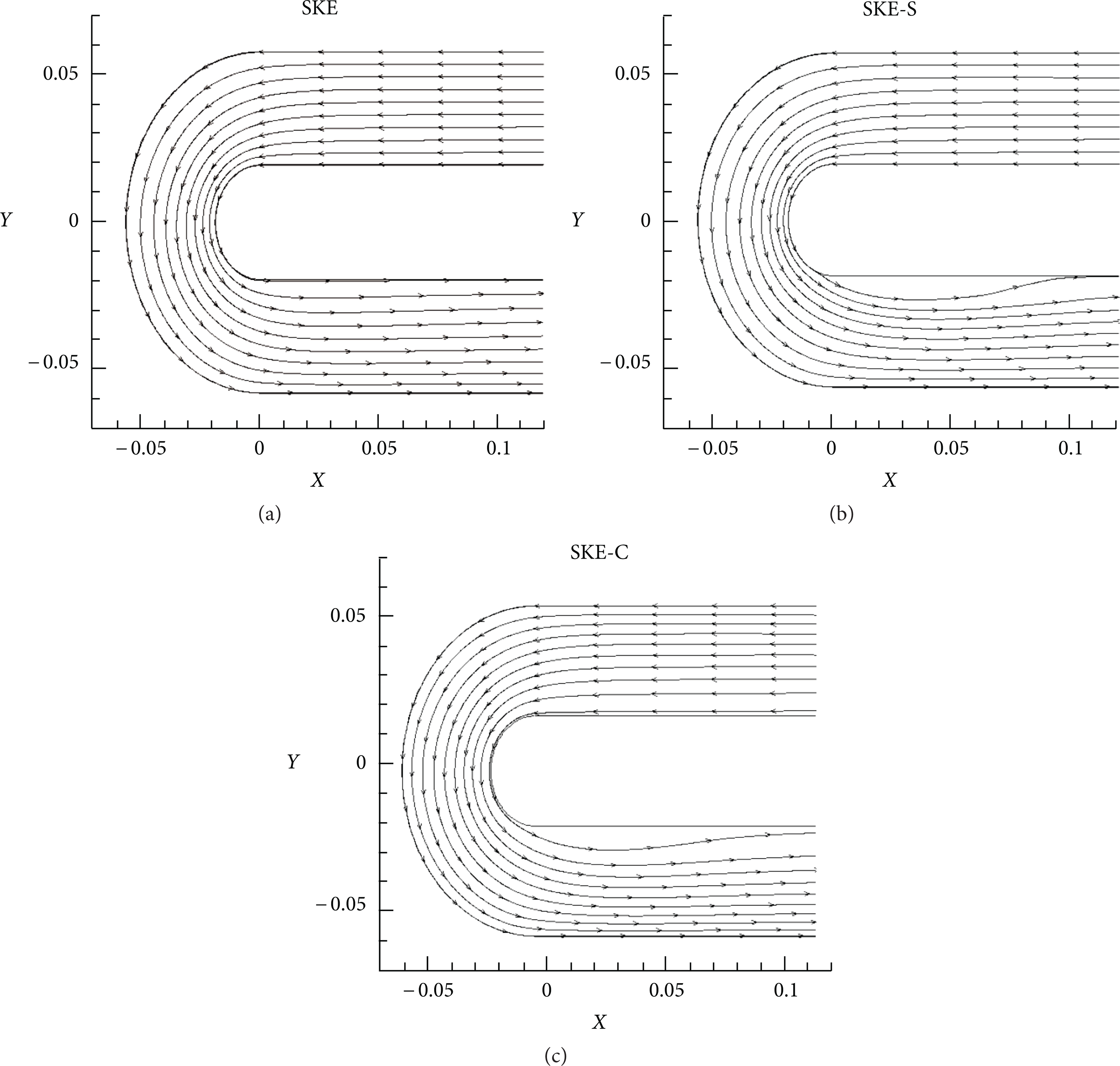
Streamlines calculated by the three models showing different sized separation bubbles in the region downstream of θ = 180°.

6. 90° Bend Flow

The flow development in a 90° bend is very similar to that in the meridional flow path of hydraulic machinery systems. In this sense, it is a useful benchmark for validation of turbulence models before being extended to applications in pumps and turbines [16]. The experimental data for this test case have been provided by the ERCOFTAC database and refer to the measurements of Kim and Patel [17] using pressure probe and hot-wire measurement techniques. The data are very detailed and cover the majority of the cross sections where major full 3D flow phenomena are developing. The advantage of the detailed measurements is that they can be used effectively as a reference for thorough validation of turbulence models.

The computational domain for this case is shown in Figure 7. The inlet is at a distance equal to 4.5H upstream of the bend, and the outlet is at a distance 30H downstream of the bend. The span extends 6H in the z-direction, with the z/H = 0 plane defined to correspond to the bottom walls. The Reynolds number is equal to 224,000, computed using the duct height H = 0.203 m and the inlet velocity U _m = 16 m/s. The grid dimensions were 172 × 138 × 132 (streamwise × spanwise × wall normal directions), which corresponds to the finest grid level tested in the study by Yakinthos et al. [18]. The value of y+ near all wall boundaries was controlled to be less than 1, which satisfies the requirements of the enhanced wall function in the two-layer k-ε model.

Figure 7:

90° bend flow geometry.

To assess the response to the secondary flow induced by the curvature, we focused on the flow development at the position located at the 45° station in the region z/H = 0.0625. The three mean velocity components were chosen for comparison between simulations and experimental data. In Figures 8–10, the coordinate direction h indicates the transverse dimension with h = 0 corresponding to the convex (outer) surface and h = 1 corresponding to the concave (inner) surface. Figure 8 shows the streamwise velocity distribution, normalized by the average velocity across the channel. The acceleration of fluid on the convex side and the deceleration on the concave side are more accurately captured by the new model, including the momentum deficit visible in the boundary layer region on the concave surface in the region h/H < 0.2. All three of the models show an overprediction of the peak streamwise velocity near the inner (convex) surface. Notably, however, the new model is better able to predict the boundary layer profile near the convex wall, resolving the reduced near-wall gradient similar to the experimental data in the region h/H > 0.9. This behavior is due to the suppression of turbulence and consequently a reduced value of the eddy viscosity, similar to the behavior shown in Figure 3.

Figure 8:

Streamwise velocity u normalized by the inlet average velocity U _m .

Figure 9:

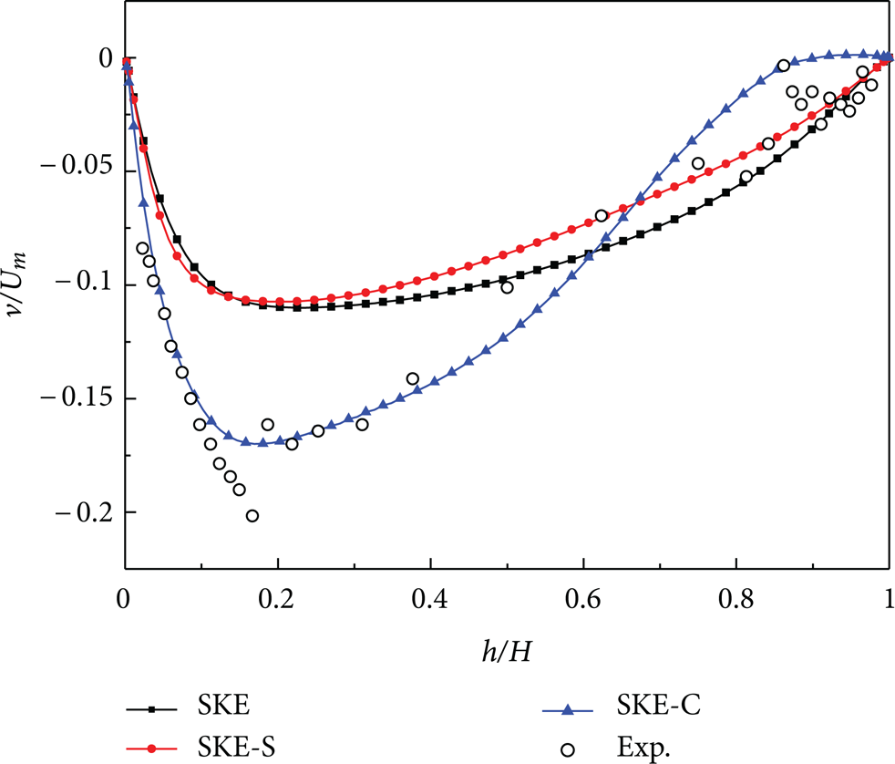
Transverse velocity v normalized by the inlet average velocity U _m .

Figure 10:

Spanwise velocity w normalized by the inlet average velocity U _m .

Figure 9 shows the normalized transverse velocity distribution which is defined to be negative in the direction from the inner side wall to the outside wall. Experiments indicate that a vortex pair is formed at this location in the channel. The effect of the vortex formation is to produce negative transverse velocity over the channel height, indicating secondary flow in the direction from the convex surface towards the inner concave surface. Among the three models tested, the SKE-C model shows this behavior most clearly, in agreement with the experimental data.

Finally, Figure 10 shows the normalized spanwise velocity distribution at this location in the channel. The large positive value near the convex surface is indicative of the secondary vortex motion. Agreement near the concave surface is good for both of the curvature corrected models; however, the behavior on the convex side (h/H > 0.6) is not well captured, with the SKE-C model indicating negative w velocity component, in contrast to the experimental data. The source of this disagreement is not clear but is almost certainly related to the underprediction of peak streamwise velocity shown in Figure 8.

7. Summary and Conclusion

This paper presents a simple eddy-viscosity formula to include sensitivity to streamline curvature and rotation effects into two-equation turbulence models. The new model is based on the work of York et al. [6], who presented a simple formula for the eddy-viscosity coefficient that included rotation and curvature effects. The new model improves accuracy over that original model by incorporating an exact calculation of local flow rotation, which is realized through the use of computed second derivatives of the mean velocity field. Stability is maintained in the new model by using a suitable level of under relaxation for the turbulent viscosity. The resulting formulation for eddy viscosity is relatively simple and satisfies principles of frame invariance and realizability.

The new model was tested on two canonical test problems for which experimental data are available for validation, and results were also compared to the standard k-ε model and to the original curvature-corrected model in [6]. For a two-dimensional U-bend flow, the new model exhibited more accurate response to streamline curvature effects, most significantly showing an improved prediction of the turbulence levels near the convex side of the channel. For the three-dimensional 90° bend flow, the new model also showed improved accuracy versus the previous model and was able to more accurately represent the effects of secondary flow in a curvature-dominated flow field. Of the three models tested, only the new model was able to correctly capture the magnitude of the transverse velocity induced by the counter-rotating vortex pair that develops in the curved section of the channel.

Results for all of the test cases indicate that the new model shows a nontrivial improvement over the original model. The model is able to qualitatively reproduce the primary effects of rotation and curvature on the Reynolds stress field, within a two-equation eddy-viscosity framework. The results presented here are encouraging but not surprising, since the model foundation has been previously validated, and the modification proposed here serves to place the model formulation on a more solid physical and mathematical footing. Furthermore, the new model, similar to the original version [6], is easily implemented into existing flow solvers since only one variable—the turbulent viscosity coefficient—needs to be modified. Due to its simplicity, realizability, and universality, it is expected that this model can provide an alternative for CFD end users for flow prediction of complex flows with significant effects of streamline curvature.