Research on Vehicle Automatically Tracking Mechanism in VANET

Abstract

The intelligent vehicle is a complex system equipped with advanced technologies such as the artificial intelligence, automatic control, and computer, communication. It is a combination of multiple academic subjects and the latest technologies representing the developing tendency of future automobile technology and attracts more and more attention. In this paper, we made some useful explorations in the fields of intelligent vehicle control technology and obstacle avoidance, and a deep research is carried out about the distance of vehicle, vehicle tracking, vehicle lane changing and intersections obstacle avoidance and communication protocols, and some innovative ideas are proposed during the research. By using VANET, some predictable status of tracing and tracking of intelligent vehicle technology was researched, and the communication protocols between two vehicles, the safe spacing algorithm, the method of computing the actual distance at corners and straights, and the trajectory of lane change were designed. In addition, a series of vehicle tracing and tracking technologies, such as without knowing the road conditions, homeostatic mechanism, keeping a safe spacing to the target vehicle, and adjusting its own speed to track the target vehicle smoothly to the destination by comparing the actual distance and safe spacing between vehicles, were discussed here.

1. Introduction

The number of vehicles owned by people is rapidly growing with the development of economy and society. The safety problem in transportation is increasingly outstanding. It brings a serious threat to humans’ life and property. As we all known, safe-driving is always one of the most important topics in vehicle engineering. In order to reduce traffic accidents, the intelligent vehicle emerges as the times require. It is a complex system equipped with advanced technologies such as the artificial intelligence, automatic control, computer, and communication. It is a combination of multiple academic subjects and latest technologies, representing the developing tendency of future automobile technology. Therefore, it attracts more and more attention. With the fast development in ad hoc wireless communications and vehicular technology, it is foreseeable that, in the near future, traffic information will be collected and disseminated in real time by mobile sensors instead of fixed sensors used in the current infrastructure-based traffic information systems. A distributed network of vehicles such as a vehicular ad hoc network (VANET) can easily turn into an infrastructure-less self-organizing traffic information system, where any vehicle can participate in collecting and reporting useful traffic information such as section travel time, flow rate, and density. Disseminating traffic information relies on broadcasting protocols [1]. In-network data aggregation is a useful technique to reduce redundant data and to improve communication efficiency. Traditional data aggregation schemes for wireless sensor networks usually rely on a fixed routing structure to ensure that data can be aggregated at certain sensor nodes [2].

Recent years have witnessed the growing popularity of sensor and sensor-network technologies, supporting important practical applications. One of the fundamental issues is how to accurately locate a user with few labeled data in a wireless sensor network, where a major difficulty arises from the need to label large quantities of user location data, which in turn requires knowledge about the locations of signal transmitters or access points [3]. Donghyun et al. considers the problem of computing the optimal trajectories of multiple mobile elements (e.g., robots, vehicles, etc.) to minimize data collection latency in WSNs [4].

A new category of intelligent sensor network applications emerges where motion is a fundamental characteristic of the system under consideration. In such applications, sensors are attached to vehicles or people that move around large geographic areas. For instance, in mission critical applications of WSNs, sinks can be associated to first responders. In such scenarios, reliable data dissemination of events is very important, as well as the efficiency in handling the mobility of both sinks and event sources. For this kind of applications, reliability means real-time data delivery with a high data delivery ratio. In their article, Erman et al. proposes a virtual infrastructure and a data dissemination protocol exploiting this infrastructure, which considers dynamic conditions of multiple sinks and sources [5]. WSNs have been increasingly available for critical applications such as security surveillance and environmental monitoring. An important performance measure of such applications is sensing coverage that characterizes how well a sensing field is monitored by a network [6]. Wireless has become one of the most pervasive core technology enablers for a diverse variety of computing and communications applications ranging from 3G/4G cellular devices, broadband access, indoor Wi-Fi networks, and vehicle-to-vehicle (V2V) systems to embedded sensor and RFID applications [7].

A large class of WSN applications involve a set of isolated urban areas covered by sensor nodes monitoring environmental parameters. Mobile sinks mounted upon urban vehicles with fixed trajectories (e.g., buses) provide the ideal infrastructure to effectively retrieve sensory data from such isolated WSN fields [8]. Jorge et al. [9] presents control and coordination algorithms for groups of vehicles. The focus is on autonomous vehicle networks performing distributed sensing tasks where each vehicle plays the role of a mobile tunable sensor. The author propose gradient descent algorithms for a class of utility functions which encode optimal coverage and sensing policies. Kwok and Martínez's work [10] includes incorporating nonholonomic vehicle dynamics into the convergence analysis in order to provide a more practical coverage scenario for implementation in a physical testbed. Since the convergence of the algorithms is only guaranteed to local optima, we are also working on extensions that help us find more optimal coverage configurations.

In this paper, we have made some positive and useful explorations in the fields of intelligent vehicle control technology and obstacle avoidance. On the basis of the current situation and the vital supporting techniques of these fields, a deep research is carried out about the distance of vehicle, vehicle tracking, vehicle lane changing, and intersection obstacle avoidance and communication protocols. Moreover, some innovative ideas are proposed during the research. Finally, a brief summary and an outlook are made about this paper.

2. The Design of Vehicle Tracing Algorithm

Many related control strategies are needed to intervene with the vehicles when they are tracked. The algorithm of control is discussed as follows.

2.1. Vehicle-to-Vehicle Safe Spacing and Minimum Safe Spacing

To avoid collision, the spacing between two vehicles must be greater than the safe spacing. Safe spacing, the distance of two vehicles for driving safely, means vehicles running in the same direction must keep the distance between one and another for the safety of traffic. Minimum safe spacing or critical safe spacing indicates the minimum intervehicle distance for safety. The capacity of roads is proportional to the velocity and is inverse proportional to the spacing of vehicles which reveals the fact that increasing the safe spacing blindly will conversely lower the traffic capacity. To keep the capacity of roads in accordance with road safety, people pay much attention to the minimum safe spacing.

The vehicle, in the motion, travels in the longitudinal direction most of time; that is, there is no transverse velocity and acceleration. So it is totally useful to study the longitudinal inter-vehicle safe spacing. As shown in Figure 1, vehicle $C_0$ and vehicle $C_1$ are running on the same lane and vehicle $C_0$ is ahead of vehicle $C_1$ . Computing the inter-vehicle safe spacing needs knowing the velocity and acceleration of both vehicles first. As it is difficult to capture both velocity and acceleration precisely, the problem demands simplification. Supposing that both of the vehicles are in condition of uniform and linear motion, the safe spacing during time 0 and $t_m$ can be computed by

$$\begin{array}{cc}& \text{MSS}=\max \left(\left(v_{\mathrm{1}}-v_{\mathrm{0}}\right)t,\mathrm{0}\right),\hspace{1em}t\in \left[\mathrm{0},t_m\right].\end{array}$$

(1)

$v_{\mathrm{0}}$ and $v_{\mathrm{1}}$ are the longitudinal velocity of vehicle $C_0$ and vehicle $C_1$ .

Figure 1

The longitudinal vehicle.

As both vehicles make uniform and linear motion, the relative velocity is always a constant, $v=v_{\mathrm{0}}-v_{\mathrm{1}}=\text{const}$ , which deduces MSS as the following rules:

$$\begin{array}{cc}& \text{MSS}=\{\begin{array}{cc}\left(v_{\mathrm{1}}-v_{\mathrm{0}}\right)t_m\hfill & v_{\mathrm{1}}-v_{\mathrm{0}}\ge \mathrm{0}\hfill \\ \mathrm{0}\hfill & v_{\mathrm{1}}-v_{\mathrm{0}}<\mathrm{0}.\hfill \end{array}\end{array}$$

(2)

In this way, there are time and minimum safe spacing. As we set different values to these parameters, series of situations and solutions are acquired as follows.

• (1)

  When relative velocity $v>0$ , inter-vehicle safe spacing will linearly increase by time. As time increases, the distance between two vehicles is getting shorter. To compensate the distance that vehicle $C_1$ travels more than vehicle $C_0$ before they collide, the MSS must be increased, so $\text{MSS}=v*t_m$ .

• (2)

  When relative velocity $v<0$ , inter-vehicle distance is increasing by time, so $\text{MSS}=\mathrm{0}$ .

• (3)

  When relative velocity $v=0$ , the MSS can be set to any value approximating to 0 in theory.

The conclusions above are based on the analysis merely considering the longitudinal minimum safe spacing preserved in advance; however, the actual distance between vehicles can not be 0. Besides the factors as relative velocity, relative acceleration and time before collision during driving, the initial velocity deserves consideration as well. The safe spacing (SS) is given by

$$\begin{array}{cc}& \text{SS}=f\left(v_{\mathrm{1}}\right)+\text{MSS}.\end{array}$$

(3)

According to (3), inter-vehicle safe spacing is a sum of critical safe spacing and a revised value. Researchers from home and abroad have put forward several models; one of them is a safe spacing model based on time interval between vehicles. The time interval (T) is defined as

$$\begin{array}{cc}& T=\frac{R}{V}.\end{array}$$

(4)

R means the relative distance between two vehicles and V means the velocity of the vehicle behind. The time interval contains the information of velocity and distance so it can demonstrate the danger level of collision. As regulations in China specify “Motor vehicles traveling on the highway must keep enough distance from the one ahead at the same lane. Under normal circumstances, when driving at 100 kilometers per hour, the safe distance is over 100 meters, when driving at 70 kilometers per hour, the safe distance is over 70 meters”. So it can be inferred that the time interval is about 3 seconds on the highway. Equation (3) can be modified as follows:

$$\begin{array}{cc}& \text{SS}=\mathrm{3}{v}_{\mathrm{1}}+\text{MSS}.\end{array}$$

(5)

2.2. Queue and Dequeue of Vehicles

The capacity of roads is proportional to the velocity of vehicles. Obviously, vehicles with great disparity of velocity driving at the same lane will lower the traffic capacity. Therefore, classifying vehicles with different velocities into different queues and putting these queues on distinctive lanes can reduce the incidence of traffic accidents to some extent. As the road sign on the highway indicates, under normal circumstances, the maximum speed is 120 kilometers per hour and the minimum speed is 60 kilometers per hour. Small passenger cars traveling on the highway shall not exceed 120 kilometers per hour, other motor vehicles shall not exceed 100 kilometers per hour, and the motorcycle shall not exceed 80 kilometers per hour. According to the regulation, there are two plans of grouping; one is based on the type of vehicles and another is based on the velocity.

Classifying vehicles with types can avoid the situation of mixing up cars and trucks and make vehicles in the same class run at the right lane. This method secures road safety as it separates motor vehicles from nonmotor vehicles. However, it is unnecessary to subdivide the vehicular road owing to the uncertain quantity of vehicles in various kinds. On the contrary, if we do so, the road capacity will probably descend. So we place emphasis on the queue of vehicles by velocities. According to the discussion above, the velocity of motor vehicles ranges from 60 kilometers per hour to 120 kilometers per hour. Supposing that the road contains at least 3 lanes, we can divide vehicles into 3 kinds of queues by velocities.

•  

  Vehicle queue 1 (C_Queue $[0]$ ), the velocity is lower than 80 kilometers per hour (km/h);

•  

  Vehicle queue 2 (C_Queue $[1]$ ), the velocity is between 80 km/h and 100 km/h;

•  

  Vehicle queue 3 (C_Queue $[2]$ ), the velocity is higher than 100 km/h.

Vehicles in specific queues run at different lanes and vehicles in the same lane are put in descending order by velocities. There are some exceptional cases in the traffic requesting disposal, such as a certain vehicle that needs changing lane or overtaking; then it comes up with the problem of regrouping the queue. During the course of regrouping, some vehicles need to leave the old queue and join a new queue. When a certain vehicle is leaving the queue, its position must be detected. When it is the head of the queue, its next vehicle is obligated to be the leader; when it is in the middle of the queue, its next one must follow the front of the leaving one; when it is the tail, it can leave the queue without any trouble. We can define a variable of Boolean type to trace the vehicle whether it is in a certain queue or not.

2.3. Vehicle Tracking

Vehicle tracking involves the mutual interaction of multiple vehicles, so the vehicle tracking model is among the interaction model. Nowadays, the interaction between intelligent vehicles is in high frequency and the complexity varies from system to system. However, the vehicle tracking model is the one much simple and deep-going. Several conditions that can track vehicles are discussed as follows.

• (1)

  The destination of the front vehicle is the same as the destination of the current vehicle.

• (2)

  The velocity of the front vehicle approximates the velocity of the current vehicle.

• (3)

  Traffic gets blocked or the lane is unchangeable and nonovertaking.

There are 3 kinds of road sections on the highway, which are straights, corners, and S-corners. As the S-corner consists of multiple corners, we simply regard the S-corner as corners. We merely take straights and corners into consideration and suppose that changing lanes is forbidden while tracking. All the vehicles are at the same lane when they are tracked, so we need to control the longitudinal direction of the vehicle rather than the transverse one to keep the velocity and safe spacing.

Most currently used vehicle tracking algorithms are safe spacing algorithms which adjust the velocity of the current vehicle to track the front vehicle by capturing images based on the visual perception technologies that record the relative position to the front vehicle. However, the complexity of the vehicle tracking algorithm on the basis of vehicle-to-vehicle and vehicle-to-roadside communications sharply diminishes compared with the visual tracking algorithm (Figure 2). After obtaining the positioning information of the front vehicle by communication, the current vehicle computes the vector difference which equals the distance between them to hold the safe spacing. It is relatively simple to apply vehicle tracking on the straight. Vehicles exchange information about positioning; velocities and so forth by communicating with each other and computing the distance L between them to keep the safe spacing. By comparing the distance with the safe spacing and regulating the velocity, vehicle tracking can be easily completed.

Figure 2

The flow diagram of the vehicle tracking algorithm.

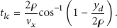
In the situation of corners, computing the distance of two vehicles by positioning is not suitable for use because the result computed now is not the actual length of the spacing but the linear distance between them. When vehicles are at the corner (the time that a deflection emerges), the spacing can be computed by knowing the velocities of both vehicles. In other words, the current vehicle captures the velocity of the front vehicle and deducts it with its own velocity, then multiplies the difference by the time during the corner. The distance L is given by

$$\begin{array}{cc}& L^{\prime }=L+\left(\left|v_{\mathrm{2}}\right|-\left|v_{\mathrm{1}}\right|\right)\mathrm{\Delta }t,\end{array}$$

(6)

where L is actual distance between two vehicles, $v_1$ is velocity of the front vehicle, $v_2$ is velocity of the front vehicle, and $\mathrm{\Delta }t$ is the time during the corner. When vehicles are at the corner, they regulate their own speed close to the velocities of other vehicles obtained by interaction to keep the safe spacing and tracking.

2.4. Lane Change of Vehicles

When a vehicle runs slower than its rear one all the time, overtaking occurs definitely with the case of lane change. Drivers need proficient skills and adequate experience when changing the lane; otherwise accidents will happen. At the very beginning of lane change, rear-end collisions are highly possible. When the distance between two vehicles is not enough, angle collisions take place likely. Figure 3 shows the sketch map of lane change. All the parameters are marked as shown in Figure 3, where $C_0$ and $C_1$ is Vehicle, L is length of the vehicle, W is width of the vehicle, θ is angle between the symmetry axis and x-axis, and $P_1~P_4$ is 4 angles of the vehicle. Establishing coordinate system as Figure 3 shows, the longitudinal acceleration, longitudinal velocity, longitudinal position, transverse acceleration, transverse velocity, and transverse position of vehicle $C_i$ are defined as $a_{ix}$ , $v_{ix}$ , $x_i$ , $a_{iy}$ , $v_{iy}$ , $y_i$ , $i\in \{\mathrm{0,1}\}$ and $x_i$ , $y_i$ means the left and front angle, such as $P_1$ .

Figure 3

The sketch map of lane change.

Lane change can be divided into several time periods. Time points of lane change are marked on the Figure 4, specifically described as shown in Figure 4, where $t_0$ is moment of starting lane change, $t_p$ is moment of collision, $t_{lc}$ is moment of finishing lane change, and T is a random time period after changing lane. Traffic in real life can be much complex, so we simplify the problem, supposing that vehicle $C_0$ does not have transverse velocity and acceleration; that is, $a_{oy}=0$ , $v_{oy}=0$ . Analyzing the relationship between the positions of two vehicles, the conditions of collision avoidance are given as follows:

$$\begin{array}{cc}& x_{\mathrm{0}}\left(t\right)>x_{\mathrm{1}}\left(t\right)+L_{\mathrm{0}}+W_{\mathrm{1}}\sin \left(\theta \left(t\right)\right)\hspace{1em}t\in \left[\mathrm{0},t_p\right].\end{array}$$

(7)

$L_{\mathrm{0}}$ means the length of vehicle $C_0$ , $\theta (t)$ means the angle between vehicle $C_0$ and x-axis at time t, and $W_{\mathrm{1}}$ means the width of vehicle $C_0$

$$\begin{array}{cc}& \theta \left(t\right)=t{g}^{-\mathrm{1}}\frac{\partial y_{\mathrm{1}}\left(t\right)}{\partial x_{\mathrm{1}}\left(t\right)}=t{g}^{-\mathrm{1}}\frac{\partial y_{\mathrm{1}}\left(t\right)/\partial t}{\partial x_{\mathrm{1}}\left(t\right)/\partial t}=t{g}^{-\mathrm{1}}\frac{v_{y\mathrm{1}}\left(t\right)}{v_{x\mathrm{1}}\left(t\right)}\end{array}$$

(8)

and setting

$$\begin{array}{cc}& S\left(t\right)=x_{\mathrm{0}}\left(t\right)-\left[x_{\mathrm{1}}\left(t\right)+L_{\mathrm{0}}+W_{\mathrm{1}}\sin \left(\theta \left(t\right)\right)\right].\end{array}$$

(9)

Figure 4

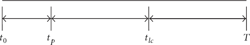
Time points of lane change.

To avoid the collision, the result of (9) is greater than 0; that is,

$$\begin{array}{l}S\left(y\right)=(S^{*}\left(\mathrm{0}\right)+{\int }_{\mathrm{0}}^t{\int }_{\mathrm{0}}^{\sigma }\left(a_{\mathrm{0}x}\left(t\right)-a_{\mathrm{1}x}\left(t\right)\right)dt\hspace{0.17em}d\sigma \\ \hspace{1em}\hspace{1em}+\left(v_{\mathrm{0}x}\left(\mathrm{0}\right)-v_{\mathrm{1}x}\left(\mathrm{0}\right)\right)t\phantom{{\int }_{\mathrm{0}}^{\sigma }\left(a_{\mathrm{0}x}\left(t\right)-a_{\mathrm{1}x}\left(t\right)\right)dtd\sigma })>\mathrm{0},\hspace{1em}t\in \left[\mathrm{0},t_p\right],\end{array}$$

(10)

$$\begin{array}{l}{S}^{*}\left(\mathrm{0}\right)=x_{\mathrm{0}}\left(\mathrm{0}\right)-L_{\mathrm{0}}-x_{\mathrm{1}}\left(\mathrm{0}\right).\end{array}$$

(11)

In order to find the minimum initial distance to avoid collisions of vehicle $C_0$ and $C_1$ , we set (11) to 0 and that means the two vehicles are end to end at the early time of lane change which can be

$$\begin{array}{l}\text{MSS}=\min ({\int }_{\mathrm{0}}^t{\int }_{\mathrm{0}}^{\sigma }\left(a_{\mathrm{0}x}\left(t\right)-a_{\mathrm{1}x}\left(t\right)\right)dt\hspace{0.17em}d\sigma \\ \hspace{1em}\hspace{0.5em}\hspace{1em}\hspace{1em}\hspace{1em}+\left(v_{\mathrm{0}x}\left(\mathrm{0}\right)-v_{\mathrm{1}x}\left(\mathrm{0}\right)\right)t\phantom{{\int }_{\mathrm{0}}^t{\int }_{\mathrm{0}}^{\sigma }\left(a_{\mathrm{0}x}\left(t\right)-a_{\mathrm{1}x}\left(t\right)\right)dt\hspace{0.17em}d\sigma })\hspace{1em}t\in \left[\mathrm{0},t_p\right].\mathrm{\hspace{0.17em}\hspace{0.17em}}\end{array}$$

(12)

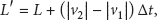
Minimum safe spacing (MSS) between the two vehicles is determined by relative longitudinal acceleration and initial velocities of the two vehicles and the time duration before collision. Lane change can have a variety of trajectories. This paper introduces the one based on the trajectory of the arc. Assuming that the vehicle lane change is divided into three stages: the initial stage of the vehicle to generate a transverse acceleration, the intermediate stage of the vehicle running straight at a constant speed, and the final stage of the vehicle to generate a transverse deceleration (the value is the same as the one in the initial stage of acceleration), as shown in Figure 5, the initial segment and the final segment of the lane change trajectory constitutes by the arc of a circle when the middle part uses straight line. The curvature of the arc radius is ρ

$$\begin{array}{cc}& \rho =\frac{v_x^{\mathrm{2}}}{a_y}.\end{array}$$

(13)

$v_x^{\mathrm{2}}$ is the longitudinal velocity of the vehicle and $a_y$ is the transverse acceleration of the vehicle.

Figure 5

The initial segment and the final segment of the lane change trajectory.

Analyzing Figure 5 can get the following:

$$\begin{array}{cc}& y_d=\mathrm{2}\rho \left(\mathrm{1}-\cos \left(\frac{v_x{t}_c}{\rho }\right)\right)+v_x{t}_l\sin \left(\frac{v_x{t}_c}{\rho }\right).\end{array}$$

(14)

The time of lane change is the sum of the time passing the both of the arc and the straight line; that is, $t_{lc}=2t_c+t_l$

$$\begin{array}{cc}& t_{lc}=\mathrm{2}{t}_c+\frac{\left(y_d-\mathrm{2}\rho +\mathrm{2}\rho \cos \left(v_x{t}_c/\rho \right)\right)}{v_x\sin \left(v_x{t}_c/\rho \right)}.\end{array}$$

(15)

Thus it can be calculated as follows:

$$\begin{array}{cc}& \frac{d{t}_{lc}}{d{t}_c}=-\frac{\left[y_d-\mathrm{2}\rho +\mathrm{2}\rho \cos \left(v_x{t}_c/\rho \right)\right]\cos \left(v_x{t}_c/\rho \right)}{\rho {\sin }^{\mathrm{2}}\left(v_x{t}_c/\rho \right)}.\end{array}$$

(16)

Setting $d{t}_{lc}/d{t}_c=\mathrm{0}$ , $t_c$ can be given as

$$\begin{array}{cc}& t_c=\frac{\rho }{v_x}{\cos }^{-\text{1}}\left(\mathrm{1}-\frac{y_d}{\mathrm{2}\rho }\right).\end{array}$$

(17)

The analysis shows that $t_{lc}$ is the function of $t_c$ . To calculate the minimum lane change time, we take the derivative of (15).

On analysis of the above equations, to make the lane change requires the least time, we can set $t_1=0$ ; that is, the time on the straight line is 0. The trajectory now consists of two sections of the same curvature arc, so

$$\begin{array}{l}{y}_d\left(t\right)\\ =\{\begin{array}{ll}\rho \left(\mathrm{1}-\cos \left(\frac{v_{x}t}{\rho }\right)\right)\hfill & \mathrm{0}\le t\le t_c\hfill \\ \rho \left[\mathrm{1}+\cos \left(\frac{v_x\left(t_{lc}-t\right)}{\rho }\right)-\mathrm{2}\cos \left(\frac{v_{x}t}{\rho }\right)\right]\hfill & t_c\le t\le t_{lc}.\hfill \end{array}\end{array}$$

(18)

The lane change time can be calculated by

$$\begin{array}{cc}& t_{lc}=\frac{\mathrm{2}\rho }{v_x}{\cos }^{-\mathrm{1}}\left(\mathrm{1}-\frac{y_d}{\mathrm{2}\rho }\right).\end{array}$$

(19)

2.5. Selection of the Road

When driving on the highway, drivers always meet the situation of vehicle shunt as shown in Figure 6. Drivers need to know the information provided by the road signs to select the road and determine the next direction of the vehicle. In this case, drivers who are not familiar with the roads often spend much time considering the problem, which inevitably reduces the traffic capacity of the road. So we assume that the road signs and driving vehicles can communicate with each other. When the distance between road signs and vehicles falls to S, they automatically establish communication. Vehicles automatically select the road according to the transmitted information to reach their destination. When there are $N\hspace{0.17em}(N>1)$ roads to reach their destinations, we can use the satellite sensors and high-precision digital map to choose the shortest one from the routes.

Figure 6

A branch of a road.

The greater the distance S when the road sign and the vehicle establish communication is, the longer time to choose the road will be. However, S cannot be infinitely large, so we limit S with a minimum distance to meet all the velocities of vehicles. Assuming that the maximum time from establishing to finishing communication is $t_m$ . After learning the route, some vehicles need to change the lane to enter the right road.

Vehicles shall be under maximum speed of 120 kilometers per hour (33.3 meters per second). To let all the vehicles successfully choose the right road, the minimum distance S is $S_{\min }$

$$\begin{array}{cc}& S_{\min }=\mathrm{33.3}{t}_m+v_x{t}_{lc}.\end{array}$$

(20)

$t_{lc}$ is the time of lane change and $v_x$ is the longitudinal velocity of the vehicle. $t_{lc}$ can be computed by the following:

$$\begin{array}{cc}& t_{lc}=\frac{\mathrm{2}\rho }{v_x}{\cos }^{-\mathrm{1}}\left(\mathrm{1}-\frac{y_d}{\mathrm{2}\rho }\right).\end{array}$$

(21)

So (20) can be replaced by

$$\begin{array}{cc}& S_{\min }=\mathrm{33.3}{t}_m+\mathrm{2}\rho \hspace{0.17em}{\cos }^{-\mathrm{1}}\left(\mathrm{1}-\frac{y_d}{\mathrm{2}\rho }\right).\end{array}$$

(22)

Nowadays, there are a variety of communication tools such as WIFI, Zigbee, Bluetooth, and infrared. After acquiring the minimum communication distance, we can choose the most suitable tool for inter-vehicle communication by the comprehensive analysis of the performance and price of those tools.

2.6. The Traffic Junction's Obstacle Avoidance Algorithm

Model cars, under the two-dimensional traffic environment, mainly need to care about the problem of the traffic junction's obstacle avoidance. The intersection can be generally divided into “T” type intersection and Cross-type intersection. “T” type intersection can be seen as part of the Cross-type intersection, so we can solve the “T” type intersection corresponding to the Cross-type intersection.

As in Figure 7, “○” signs are the highly possible positions in which two vehicles traveling along two different directions may collide. In order to prevent collisions between vehicles, the velocity of the vehicle needs control so that the vehicle can pass the road crossing point in an order which can effectively solve the problem of the traffic junction's obstacle avoidance.

Figure 7

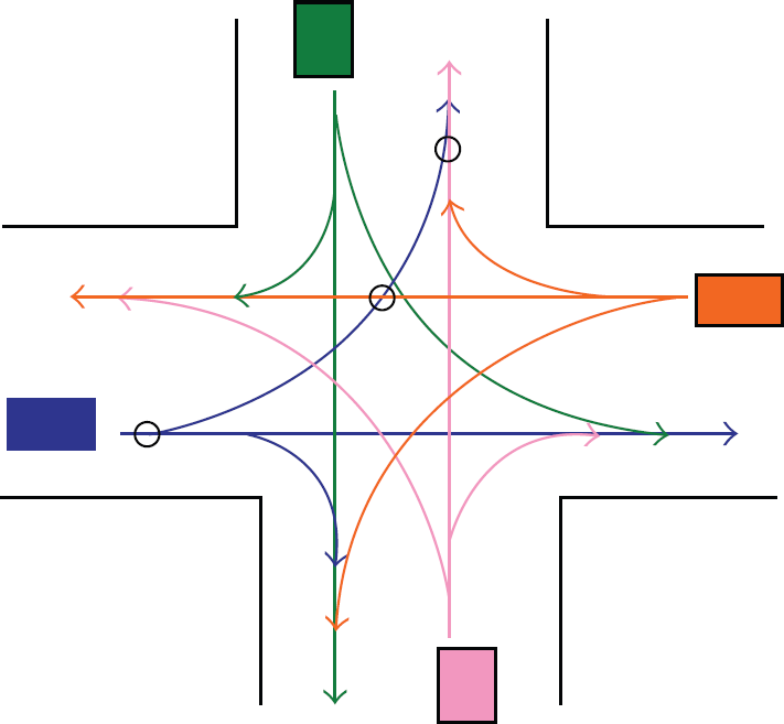
“T” type and Cross-type intersection.

Establish a certain area as the intersection point management control region (region III and within the region shown in Figure 8) around the road crossing point (i.e., the “○” symbols). Form a queue of sequent vehicles driving into the region and control the vehicles at low speed. When the vehicle is in the most forward position in the queue, it can be permitted to travel through the crossing point at full speed. Arrange a security area in the region (region I in Figure 8) which allows only one vehicle at the same time. Outside the security area is a parking area (region II in Figure 8) in which vehicles driving through can immediately stop when there is a vehicle in region I.

Figure 8

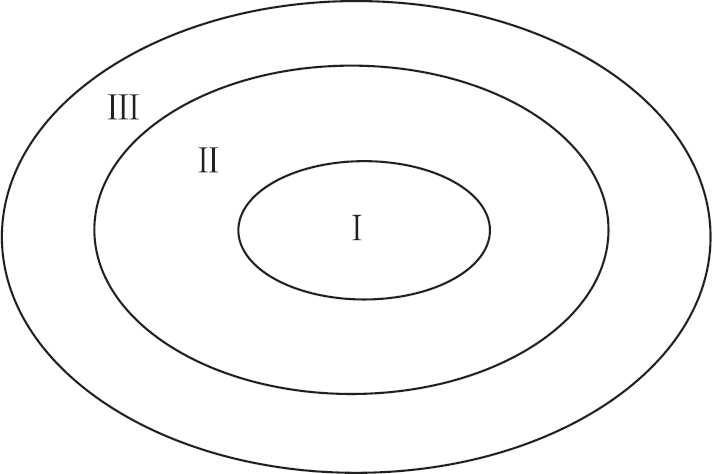
The disjunctive security regions.

When a vehicle enters the region I, the vehicle sends instructions to inform other vehicles that the intersection resource is occupied. Other vehicles receive this instruction and immediately reduce their speed to ensure they can stop outside region I. When the vehicle passes the crossing point, it needs to send instructions to inform other vehicles that there is no vehicle in region I and other vehicles take actions based on the positioning information. If the distance between the region and the certain vehicle is the shortest, then it starts to move, enters region I and sends instructions. This cycle is repeat. When the vehicle in motion does not receive any instructions, indicating that the road is clear, it can go through the road crossing point directly.

This intersection avoidance algorithm provides an effective method of traffic junction's management. It not only can let vehicles pass through the junction safely, but also change the traditional thought of controlling vehicles to run or wait by traffic lights.

3. The Communication Protocols between Two Vehicles

There must be a communication between two vehicles to complete the tracing and tracking. This section introduces the methods of the communication protocols, the provisions of transmission protocols, and feedback protocols. Finally, dynamic simulation of sending and receiving messages is carried out to verify the function of the protocols.

3.1. Pulse Width Modulator (PWM)

At present, many communication tools can be put into use, but none of them meet the requirements of the intelligent vehicle as lack of communication protocols [11].

PWM is an abbreviation of the “Pulse Width Modulation.” Its principle is using the digital output of the microprocessor to control the analog circuits by changing the pulse width to control the output voltage and changing the cycle of the pulse modulation to control the output frequency. It is frequently used in the field of measurement, communication, control, and power transform. PWM is different with some other technologies. It uses the high-resolution counters to modulate the duty cycle of the square wave and encodes the analog signals with numeric characters. Because at any moment, the DC power supply of the full amplitude only can be placed in one of the two cases on (ON) and off (OFF), the property of the PWM signal is digital, remaining unchanged. Current source or voltage is applied to the analog load in an on (ON) or off (OFF) repetitive pulse sequence. When it is on (ON), DC power supply is operating. When it is off (OFF), DC power supply is cut off.

PWM can be used to control the coding of the command word. Sending pulses of varying width represents different meanings. The receiver can use a timer to measure the pulse width. The timer is activated by the beginning of the pulse and deactivated when the pulse ends; thereby the elapsed time and the certain command can be determined. Therefore, we can use this function of PWM to specify the communication protocols to help the vehicle system establish effective communication and complete the tracing and tracking of the model car.

PWM generates a repeated alternately output signal between high level and low level, that is, the PWM wave, which specify the required clock period and duty cycle to control the duration of the high and low. Duty cycle refers the percentage of the time that the signal is at high level to the whole signal cycle and the time is determined by the pulse width. Therefore, we can set a fixed signal cycle to the PWM wave and specify the vehicle interactive communication protocol using different pulse width setting by different duty cycle.

Figure 9 describes three different PWM signals. (a) shows a 10% duty cycle PWM output, that is; 10% of the entire signal cycle is on and the remaining 90% of the time is off. (b) and (c) show, respectively, the duty cycle of the PWM output of 50% and 90%. These three PWM output encodes represent three different analog signal values at the strengths of 10%, 50%, and 90% to the full scale. For example, assuming that the power supply is 9 V and the duty cycle is 10%, the corresponding analog signal is 0.9 V.

• (1)

  Signals from the processor to the system are in digital form which means DA/AD converter is no longer needed and the impact of noise can be reduced to a minimum. Signal stored in digital form is particularly strong to resist the noise. Only when the noise is big enough to change logic 1 to logic 0 or change logic 0 to logic 1, the digital signal can be interfered.

• (2)

  It can greatly extend the communication distance. Based on this advantage, the PWM sometimes can be used for communication between two vehicles.

Figure 9

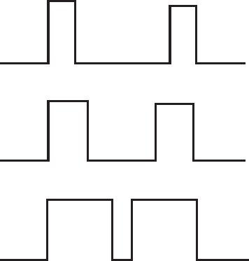
The three different PWM signals.

3.2. The Definition of the Transmission Protocol

The communication between two vehicles must be controlled by messages. Messages shall not be disorganized but shall obey some kinds of rules. Since these rules have not been defined yet in the field of vehicle research, we need to specify them.

Considering that there are many protocols used for the communication between vehicles, we define the length of the message transmission protocol as 4 bytes, totally 32 bits, to ensure that each protocol can be defined and newly found protocols can be added as well.

Errors may occur during the process of message transmission, so receivers may get wrong messages as a result. In order to make the receiver distinguish which messages are wrong, the bit at the end of the last byte is used for error checking. The check method is “XOR”; that is, xor the first 31 bits. If the result is the same as the last one, it means no error occurs in the message transmission process and the received message is correct; otherwise error occurs during the transmission, the received message is wrong, and the sender is required to retransmit the message. The last bit of the message from the sender is the result of xor'ing its first 31 bits.

3.2.1. The Types of the Message Transmission

Many actions may occur when the vehicle is traveling on the road such as the ascent or descent, left turning or right turning. These actions are the message that we need to formulate. To make these message more specific, we classify them into the following types.

(1) Velocity Transmission. When a vehicle is tracking another one, the distance between them shall be monitored from time to time in order to prevent end-to-end collisions. To compute the safe spacing, the velocities of the two vehicles are needed. One of the vehicles can get its own velocity by the sensor and get the other one's velocity by transmission. Therefore the transmission rate protocol is obviously necessary.

(2) Left or Right Turning. Vehicles may face the situations of turning a corner or turning round when they are traveling on the road. They need to turn left or right to continue moving forward on these occasions. In order to track the vehicle ahead successfully, the following one needs to be informed of the detailed messages including the degree of turning. So it is important to specify the left or right turning protocol.

(3) Acceleration and Deceleration. Vehicles will certainly be in the process of acceleration or deceleration, so the acceleration and deceleration protocol is needed to be established. When a driver starts a vehicle, he generally shifts into first gear and steps the throttle to accelerate. When the vehicle reaches a speed of 15 kilometers per hour, it is upshifted into second gear. If the driver needs acceleration, he simply inputs some gas by pressing the accelerator. When the vehicle reaches a speed of 30 kilometers per hour, it is upshifted into third gear. If the driver still needs acceleration, he speeds the vehicle up by the accelerator. When the vehicle reaches a speed of 40 kilometers per hour, it is upshifted into fourth gear. After that if acceleration is still needed, the drive keeps pressing the accelerator until the vehicle reaches the desired speed. Deceleration is implemented by downshifting and braking to be introduced next.

(4) Braking. Vehicles have to brake in case of emergency. Depending on the degree of emergency cases, the levels of brake are also different. In this paper, brake can be divided into four levels. Level 1 is sudden brake; the brake pedal is pushed to the floor with the fastest speed. Level 2 is intermediate brake; the brake pedal is pushed to two-thirds. Level 3 is light brake; the brake pedal can be pushed to one third. Level 4 is the lightest brake; use the first half of the brake pedal that is designed to be soft and push it slightly with the clutch.

(5) Overtaking. There are more than two vehicles in road traffic and there may be other vehicles inserted between them; of course they will also overtake other vehicles. When the distance between the two vehicles is large enough and the front vehicle is slower than the rear vehicle for a long time, the driver in the rear one can consider overtaking. The vehicle being tracked shall send messages to the following vehicle when it successfully finishes overtaking so as to indicate the following vehicle to overtake successfully as well.

(6) Front Road Status. Owing to the tracer which is following the front vehicle, the tracer will be blind to the road traffic if the front vehicle does not inform it. The road traffic ahead can be described as “Road Construction Ahead,” “Traffic Jam Ahead,” and “Rest Area Ahead.”

(7) Emergency. Vehicle will encounter all sorts of unexpected situations, such as the front vehicle getting a flat tire, traffic accidents ahead, keeping intervehicle spacing and the front vehicle getting flameout, and so forth.

(8) Ascent or Descent. When the driving road is not flat, it always comes with ascents or descents. The front vehicle transmits messages to the tracer during ascents or descents and tells the tracer about the probable angle of the slope so that the tracer can track the front vehicle without any trouble.

(9) Road Condition. The vehicle being tracked needs to transmit messages to its tracer whether it is at the corner or the straight. This protocol is used to transmit messages like this.

(10) Other. In addition to the previous protocols, other protocols also exist; for example, the vehicle being tracked has arrived in destination, the target being tracked and the tracer switch roles, and so forth.

3.2.2. The Codes and Regulations of the Message Transmission

(1) Velocity Transmission. The current 2 bytes and the first 4 bits of the third byte are all 0 which represent sending the velocity of the vehicle; the unit of the velocity is km/h; the last 4 bits of the third byte and the first 7 bits of the fourth byte describe the velocity in binary representation, for example: 00000000000000000000000100000111 on behalf of the vehicle at a speed of 67 kilometers per hour.

(2) Left or Right Turning. The codes of left or right turning message are shown in Table 1.

Table 1

The turning message.

00000000	00000000	00010000	00000001	Turn left and the angle is less than or equal to 1°
00000000	00000000	00010000	00000010	Turn left and the angle is between 1° and 2°
00000000	00000000	00010000	00000100	Turn left and the angle is between 2° and 3°
⋮	⋮	⋮	⋮	⋮
00000000	00000000	00010000	00001000	Turn right and the angle is less than or equal to 1°
00000000	00000000	00010000	00001011	Turn right and the angle is between 1° and 2°
00000000	00000000	00010000	00001101	Turn right and the angle is between 2° and 3°
⋮	⋮	⋮	⋮	⋮

Some details such as checkouts and security were leaved out here.

3.2.3. The Codes and Regulations of the Error Message Transmission

(1) Errors Occur in the Process of Transmission. The vehicle being tracked transmits the correct message, but an error occurs in the process of transmission; that is, one bit or several bits of the message change from 0 to 1 or from 1 to 0, so that the tracer figures out that the message is incorrect after receiving and checking it. Then, the tracer shall respond to the message as “Transmission error, please resend!”

The vehicle being tracked transmits an error message itself, that is, the result of xor'ing the first 31 bits is not equal to the last bit. Then, the tracer shall respond with the message as “Transmission error, please resend!”

(2) The Message Does Not Belong to a Certain Type. As there are various kinds of messages, we classify these message into different types to make them easy to remember, such as left or right turning message and ascent or descent protocol. We design a page for each type, when transmitting the message that is uncorrelated with the certain page; the page cannot receive it. The tracer shall respond to the message as “The message does not belong to this type, please resend!”

(3) The Message Has Not Been Defined. As the length of the message is defined as 4 bytes, totally 32 bits, the code space still has much room to use. When the vehicle being tracked sends the code that is not corresponding with any actions, the tracer shall respond to the message as “The message has not been defined, please resend!”

3.2.4. The Definition of Feedback

The tracer replies to the vehicle being tracked after receiving the message to tell if the message is received correctly or if it is necessary to resend the message. The message sent back by the tracer is called feedback. The length of feedback is 4 bytes, 32 bits. The feedback protocol is more simpler than the transmission protocol; it is mainly divided into the following types.

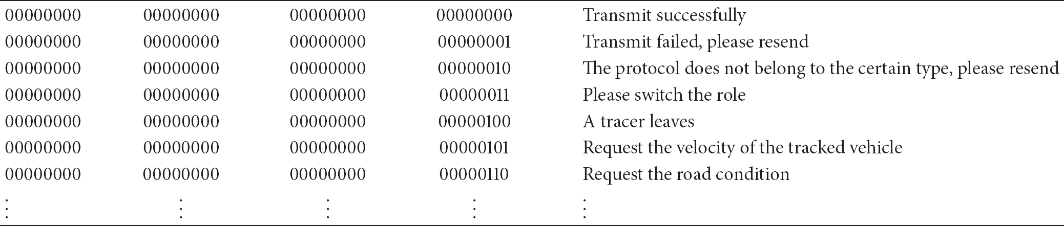
(1) Transmit Successfully. If the tracer receives messages from the vehicle being tracked correctly, the feedback is “Transmit successfully!”

(2) Transmit Failed, Please Resend. The vehicle being tracked transmits an error message itself; that is, the result of xor'ing the first 31 bits is not equal to the last bit. The feedback is “Transmission failed, please resend!”

(3) The Message Does Not Belong to a Certain Type, Please Resend. When the tracer receives the message that is not corresponding to the certain type, the feedback is “The message does not belong to the certain type, please resend!”

(4) Please Switch the Role. When the vehicle being tracked transmits the message of switching the role, the tracer replies with the feedback “Please switch the role of tracer!” and informs the vehicle to slow down.

(5)  A Tracer Leaves. When a tracer is about to leave the queue, the tracer shall send the message “A tracer leaves!” to let the vehicle being tracked know the situation.

(6) Request the Velocity of the Tracked Vehicle. When it comes to the case of computing the safe spacing between two vehicles at a certain time, the velocity of the tracked vehicle is needed and the tracer can send the message “Request the velocity of the tracked vehicle!” to get the information.

(7) Request the Road Condition. The vehicle being tracked needs to transmit messages to its tracer whether it is at the corner or the straight so as to compute the safe spacing between them. The tracer needs to send the message; that is, “Request the road condition!”

3.2.5. The Codes and Regulations of the Feedback

The codes of feedback message are shown in Table 2.

Table 2

The codes of feedback protocol and its significations.

00000000	00000000	00000000	00000000	Transmit successfully
00000000	00000000	00000000	00000001	Transmit failed, please resend
00000000	00000000	00000000	00000010	The protocol does not belong to the certain type, please resend
00000000	00000000	00000000	00000011	Please switch the role
00000000	00000000	00000000	00000100	A tracer leaves
00000000	00000000	00000000	00000101	Request the velocity of the tracked vehicle
00000000	00000000	00000000	00000110	Request the road condition
⋮	⋮	⋮	⋮	⋮

The security and validation of the protocol can refer to the relevant sections of the existing mobile network protocols and are no longer discussed in this paper [12].

4. Conclusion

This paper mainly talks about the vehicle tracing and tracking mechanism automatically. By learning the vital supporting techniques of intelligent vehicles, we discuss how to smooth the situations that the intelligent vehicle meets and design algorithms to solve part of the problems on the combination of these techniques and the traffic conditions. This paper concentrates not only on a single vehicle, but also on the mutual interaction of multiple vehicles concerning vehicle tracking and intersection obstacle avoidance. As it refers to intersection obstacle avoidance, the tradition of controlling vehicles to run or wait by traffic lights at crossroads has been altered by a new thought that vehicles contact each other and exchange the messages of the “occupied” or “released” state of the road resource at junctions. Furthermore, the research on vehicle communication protocols is a huge breakthrough. Although applying wireless communication technologies to intelligent vehicles has been mentioned by domestic researchers many times, none of them make a detailed definition of the vehicle communication protocols.