Data Storage Scheme Supporting for Multidimensional Query

Abstract

The query and storage of data is very important in wireless sensor networks (WSN). It is mainly used to solve how to effectively manage the distributed data in the monitored area with extremely limited resources. Recent advances in technology have made the number of the sensing modules in one sensor develop from single to multiple. The existing storage scheme for one-dimensional data is not suitable for the multidimensional data or costs too much energy. We proposed a kind of data storage scheme supporting multidimensional query inspired by K-D tree. The scheme can effectively store the high-dimensional similar data to the same piece of two-dimensional area. It can quickly fix the storage area of the event by analyzing the query condition and then fetch back the query result. Meanwhile the scheme has a certain degree of robustness to packet loss and node failure. Finally the experiment on the platform of Matlab showed that our scheme has some advantages compared with the existing methods.

1. Introduction

A wireless sensor network is composed of a large number of sensor nodes deployed in the monitored area and these nodes communicate through wireless waves. The basic function of WSN is accessing the information. The user can get the information of objects through these nodes and can even control some of them [1].

As the basic component of WSN, a sensor node usually consists of several modules, just like sensing module, processing module, communication module, and power module [2]. Earlier sensor node is simple and usually includes only one sensor, such as temperature sensor or humidity sensor. It gets only one numerical value when it detected events and these events are called one-dimensional events. The queries for these events are called one-dimensional query. Recent advances in technology have made the number of sensor of the sensing model develops from single sensor to multiple sensors and the sensing model can get several numerical values at the same time, such as temperature, humidity, light, and pressure. When it detects an event, it gets a value like $〈$ temperature, humidity, light, pressure $\dots 〉$ and these events are called multidimensional events. According to the number of dimensions and the range size of query, multidimensional query can be divided into multidimensional exact match point query, multidimensional partial match point query, multidimensional exact match range query, and multidimensional partial match range query [3].

Multidimensional events emerge with the development of technology. The existing data storage schemes are designed for the one-dimensional event and these schemes cannot be used for multidimensional event, or it costs too much energy in multidimensional event query. Limited energy is an important feature of WSN and the life time of the whole network is an important indicator of its performance; meanwhile the long-time stable running is also a significant security for the usage in reality. So how to design a data storage scheme to support the multidimensional query, which can avoid amount of useless queries, reduce the response time, save the energy of the nodes, and extend the life of the network, is faced by all scholars.

The existing schemes supporting for multidimensional query include DIM [4] and Pool [5]. DIM is the first algorithm used to solve the problem. It stores the event by using the code of the event and resolves the query into many subqueries and gets the result, respectively. Pool addresses some weakness of DIM such as hot spot and scalability problems and further proposes a storage scheme to group index nodes together as a data pool to preserve the neighborhood property of nearby multidimensional data; however, their group mechanism is only based on the greatest and the second greatest attribute values, which has not been proved to be efficient enough for high-dimensional data processing. The literature [6] proposed a secure and reliable data distribution scheme in unattended WSNs. Work [7] proposed an energy-efficient query algorithm to query the top-k value of sensed data. MDCS is a multiresolution data compression and storage strategy [8]. Work [9] proposed a bouncing-track-based data storage and discovery scheme in WSN. The literature [10] proposed a secure and reliable data distribution scheme in WSN.

The existing storage schemes supporting multidimensional query mainly give solutions from the theoretical point, but there are still many shortcomings. Hot spots: the storage node and the nodes nearby may quickly become the hot spots because of excessive communication. Scalability problem: as the number of sensor nodes in the system increases, the amount of message exchanges among sensors increases too fast. Query costs too much: the cost is too high in the present schemes. Hard to implement: most of the existing schemes require the accurate division of the network to ensure a grid only has only one or a few nodes and this is hard to carry out in real [11].

Faced with the emergence of the multidimensional events and flaws of the existing data storage schemes, we propose a new method inspired by K-D tree. It can solve the flaws in some degree, effectively reduce the energy cost, and extend the life of the network.

2. Design of Data Storage Scheme Supporting for Multidimensional Query

2.1. K-D Tree Introduction

K-D tree [12] is a data structure that can effectively store multidimensional data. K represents the dimensionality of the search space; K-D tree is evolved from the binary tree. The difference is that each layer represents a dimension and you can use the value of each dimension as a splitter to make decisions. The top layer node is chosen from any of the k dimensions. The second layer is divided by another dimension. When the value of depth of the tree is larger than the value of dimensions, you can reuse these dimensions.

The advantage of the K-D tree is that the data are classified according to the value of each dimension. The closer the value of each dimensional data the more probable the data may be classified together, this idea can be directly applied to multidimensional queries in WSN. In the progress of designing the data storage supporting multidimensional querying, first, you should map the data in high-dimensional space to two-dimensional space and maintain the local nature [13]. Second, you can reuse the dimension to split the data into smaller range. So you can give a more accurate position in querying. Third, you can split the area according to each value, and this value also can be applied to the division of monitoring area in WSN.

The basic idea of data storage is as follows: suppose the dimension of monitored event is k; first, we construct a binary tree of depth of d, $d⩾k$ . Each layer of the tree is corresponded to each dimension of the event. When $d⩽k$ , each layer of the tree is divided according to 0.5. When $k⩽d⩽2k$ , 0.25 and 0.75 are used as the splitter values. At last all data are stored in leaf nodes.

2.2. Data Storage Mechanism

2.2.1. Mapping an Event to a Storage Area

Suppose the wireless sensor nodes are uniformly distributed in the monitoring area, and nodes can communicate through the exchange of information. All nodes know their coordinates in the area. When the node detects an event, it will get a set of data elements about the event. We use E to represent the k-dimensional event: $E=〈V_1,V_2,\dots ,V_k〉$ , in which each attribute value has normalized. For the query issued by the user, we use Q to represent $Q=〈[L_1,U_1],[L_2,U_2],\dots ,[L_h,U_h]〉$ , $h\le k$ ; in which $L_i$ and $U_i$ , respectively, represent the minimum and maximum attributes of i.

First, we construct a virtual binary tree before mapping the event to the storage area, then we divide the storage area and insert event on the basis of the binary tree. The key point is how to fix the depth of the tree, because it will decide the number of storage area. Assume the depth of the tree is d and the dimension of event is k. To each dimension of events for a comparison, the depth needs to fix the condition: $d⩾k$ . For the maximum value about d, we assume nodes in each partitioned grid will receive the data in all directions and have the same probability. In order to store data with the best balanced manner, we set a storage node in each direction, so the grid should have at least 8 nodes. Assume the number of nodes in the network is N, so the number of grid is $N/8$ at most and the maximum depth of the tree is $d\le \sqrt{N/8}$ . Therefore, the depth of the tree should meet the condition: $k\le d\le \sqrt{N/8}$ . The value of d can be flexibly selected according to the size of monitoring area.

When the depth of the tree d is determined, the network monitoring area is divided into $2^d$ storage area. When the event is generated in the network, it should be stored into appropriate storage area. First, we should encode the event. For event $E=〈V_1,V_2,\dots ,V_k〉$ , we assign a d-bit binary string. For every bit i, i changes from 1 to k; if $0\le V_i<\mathrm{0.5}$ , this bit is encoded as 0; if $\mathrm{0.5}\le V_i\le 1$ , this bit is encoded as 1. When i changes from $k+1$ to $2k$ , if $(0\le V_{i-k}<\mathrm{0.25})\cup (\mathrm{0.5}\le V_{i-k}<\mathrm{0.75})$ , this bit is encoded as 0; if $(\mathrm{0.25}\le V_{i-k}<\mathrm{0.5})\cup (\mathrm{0.75}\le V_{i-k}\le 1)$ , this bit is encoded as 1. This work stops until the d-bit numbers are all assigned. At last, the event E is encoded into $E_{\text{code}}$ .

In $E_{\text{code}}$ , the odd bit divides the area symmetry in left and right. Left is 0 and right is 1. The event bit divides the area into above and below. Above is 0 and below is 1. So each binary string at last determines a storage area. This storage area is defined by the lower left coordinates $(X_{\text{low}},Y_{\text{low}})$ and upper right coordinates $(X_{\text{up}},Y_{\text{up}})$ .

Suppose $E_{\text{code}}=[x_1,y_1,x_2,y_2,\dots ,x_{d/2},y_{d/2}]$ ; we first calculate the lower bound $X_{\text{low}}$ on the x-axis as follows:

$$\begin{array}{cc}& X_{\text{low}}=x_1\left(\mathrm{0.5}\right)+x_2{\left(\mathrm{0.5}\right)}^2+\cdots +x_{d/2}{\left(\mathrm{0.5}\right)}^{d/2}.\end{array}$$

(1)

We get the lower bound of y-axis as follows:

$$\begin{array}{cc}& Y_{\text{low}}=y_1\left(\mathrm{0.5}\right)+y_2{\left(\mathrm{0.5}\right)}^2+\cdots +y_{d/2}{\left(\mathrm{0.5}\right)}^{d/2}.\end{array}$$

(2)

Therefore we define a matrix M as follows:

$$\begin{array}{cc}& M=\left[\begin{array}{cc}\left(\frac{1}{2}\right)& 0\\ 0& \left(\frac{1}{2}\right)\\ {\left(\frac{1}{2}\right)}^2& 0\\ 0& {\left(\frac{1}{2}\right)}^2\\ {\left(\frac{1}{2}\right)}^{d/2}& 0\\ 0& {\left(\frac{1}{2}\right)}^{d/2}\end{array}\right].\end{array}$$

(3)

We can calculate $R_{\text{low}}$ as follow:

$$\begin{array}{cc}& R_{\text{low}}=\left[X_{\text{low}},Y_{\text{low}}\right]=E_{\text{code}}·M.\end{array}$$

(4)

After getting the lower bound of the storage area, we need to find the upper bound $X_{\text{up}}$ and $Y_{\text{up}}$ . We first make XOR operation on $E_{\text{code}}$ :

$$\begin{array}{cc}& \overline{E_{\text{code}}}=E_{\text{code}}\oplus J_d\hspace{1em}{J}_{d/2}={\left[\mathrm{1,1},\dots ,1\right]}_{1\times d}.\end{array}$$

(5)

Then we calculate $\overline{R_{\text{up}}}$ :

$$\begin{array}{cc}& \overline{R_{\text{up}}}=\left[\overline{X_{\text{up}}},\overline{Y_{\text{up}}}\right]=\overline{E_{\text{code}}}·M.\end{array}$$

(6)

At last we calculate the real upper bound $R_{\text{up}}$ :

$$\begin{array}{cc}& R_{\text{up}}=\left[X_{\text{up}},Y_{\text{up}}\right]=J_2-\overline{R_{\text{up}}}.\end{array}$$

(7)

Finally the storage area is defined by $R_{\text{low}}$ and $R_{\text{up}}$ : $R=[X_{\text{low}}~X_{\text{up}},Y_{\text{low}}~Y_{\text{up}}]$ .

2.2.2. Routing an Event to a Storage Area

After getting the storage area of an event, we need to route the event to this area to store. The progress is as follows: the node that detected the event first compares its geographic coordinate with the coordinate of storage area. If the node's coordinate falls in the range of storage area's coordinate, the node will store the event locally. Otherwise, the node will attempt to route the event to the corresponding storage area with GPSR (GPSR: Greedy Perimeter Stateless Routing for Wireless Networks).

GPSR is a geographic routing protocol, the benefit of which is that it can route the packet to the destination with greedy manner after known coordinate of the source node and destination node [14]. In addition to the protocol's own information, the package also carried the coordinate of the storage area. The packet format is as follows:

$\begin{array}{cccccccc}\text{ID}& \cdots & X_{\text{low}}& Y_{\text{low}}& X_{\text{up}}& Y_{\text{up}}& X_{\text{mid}}& Y_{\text{mid}}.\end{array}$

$X_{\text{mid}}$ and $Y_{\text{mid}}$ represent the coordinate of the center of R. They are the destination address of GPSR. In the routing progress, every node will compare its own coordinate with them. When a node meets the condition of $(X_{\text{low}}\le x\le X_{\text{up}})\hspace{0.17em}\cap \hspace{0.17em}(Y_{\text{low}}\le y\le Y_{\text{up}})$ , that means the event has been routed to the storage area. The next step is selecting a node to store the event. In order to ensure load balancing, the selection of storage nodes needs to meet certain conditions.

2.2.3. Load Balance in the Storage Area

After the event has been routed to the storage area, we need to select a node to store the event. There are many methods. In this scheme we operate like this: we select the node along the direction of the event coming from and closest to the center of the area to store as Figure 1 shows. Suppose the lower left coordinate of R is $R_{\text{low}}(X_{\text{low}},Y_{\text{low}})$ , the upper right coordinate of R is $R_{\text{up}}(X_{\text{up}},Y_{\text{up}})$ , and the middle coordinate of R is $R_{\text{mid}}(X_{\text{mid}},Y_{\text{mid}})$ ; then the storage node $S(x,y)$ should meet the following condition: $\mathrm{Min}\sqrt{(x-X_{\text{mid}}{)}^2+(y-Y_{\text{mid}}{)}^2}$ and $(X_{\text{low}}\le x\le X_{\text{up}})\cap (Y_{\text{low}}\le y\le Y_{\text{up}})$ .

Figure 1

Load balance in storage area.

The storage capacity of every node in the network is limited. We set a threshold to node's memory load. When the capacity of the node reaches the threshold, the node cannot receive events. In the progress of selecting storage nodes, the node will be skipped. By using this method, every node will have the opportunity to store events.

2.3. Data Query Mechanism

The query processing mechanism contains two parts: query resolving and retrieval route. The design of the query resolving is determining a set of relevant range spaces which can provide answers to the query. The retrieval route is fetching match events to the query from set space.

2.3.1. Query Resolving

Multidimensional queries include point queries and range queries. Point querying is identical to inserting an event, but range querying includes multidimensional exact match range querying and multidimensional partial match range querying. It is related to more storage areas, so you need to resolve the query conditions first. The following parts, respectively, described their solutions.

(1) Query Resolving Mechanism for Exact Match Range Queries

We represent the event in the network with $E=〈V_1,V_2,\dots ,V_k〉$ , when the user sends a query like $Q=〈[L_1,U_1],[L_2,U_2],\dots ,[L_h,U_h]〉$ and it satisfies $(h=k)\cap (L_i\le U_i)$ , $1\le i\le k$ . We call the query as exact match range querying. How to split the query is as follows: if the depth of the binary tree is identical to the number of dimensions, then we check Q's ith attribute whether contains the value 0.5. If it contains, then we divide the Q in two subqueries. If the depth is larger, then the query will be divided into smaller ranges. For example, if you send a query $Q=〈[\mathrm{0.3,0.6}],[\mathrm{0.7,0.8}],[\mathrm{0.3,0.4}]〉$ and the depth of the binary tree is 4, you will get four subqueries after resolving:

$$\begin{array}{cc}& Q_1=〈\left[\mathrm{0.3,0.5}\right),\left[\mathrm{0.7,0.8}\right],\left[\mathrm{0.3,0.4}\right],\left[\mathrm{0.3,0.5}\right]〉,\\ Q_2=〈\left[\mathrm{0.3,0.5}\right),\left[\mathrm{0.7,0.8}\right],\left[\mathrm{0.3,0.4}\right],\left[\mathrm{0.5,0.6}\right]〉,\\ Q_3=〈\left[\mathrm{0.5,0.6}\right],\left[\mathrm{0.7,0.8}\right],\left[\mathrm{0.3,0.4}\right],\left[\mathrm{0.3,0.5}\right]〉,\\ Q_4=〈\left[\mathrm{0.5,0.6}\right],\left[\mathrm{0.7,0.8}\right],\left[\mathrm{0.3,0.4}\right],\left[\mathrm{0.5,0.6}\right]〉.\end{array}$$

(8)

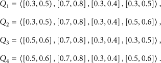
The binary strings of the four subqueries are 0101, 0100, 1101, and 1100 and they, respectively, correspond with four storage areas in the network. 0101 and 0100, 1101 and 1100 are different with the last bit. We can certify their storage areas are adjacent. So if sub-queries are just different with the last bit, we can combine the two sub-queries into one query and get rid of the last bit. In this example, the combined binary strings are 101 and 110. The benefit of the mechanism is reducing the number of routing path from four to two to save the power energy.

(2) Query Resolving Mechanism for Partial Match Range Queries

Assume that $Q=〈[L_1,U_1],[L_2,U_2]〉=〈[\mathrm{0.3,0.6}],[\mathrm{0.7,0.8}]〉$ is a three-dimensional partial match range query. The value of the three-dimensional can be anything. That means there are more results satisfing the condition and the searching area for the query will be extended. For this kind of queries, we can reset the range of each unspecified attribute as $[0,1]$ , then the query became $Q=〈[\mathrm{0.3,0.6}],[\mathrm{0.7,0.8}],[\mathrm{0,1}]〉$ , then we can use the resolving method of exact match range queries.

2.3.2. Retrieval Route

Routing queries is similar to inserting an event. You can get several sub-queries after resolving and combining these queries. And every binary string of the sub-queries corresponds to a storage area. By using GPSR routing protocol, these sub-queries will route to their corresponding storage areas. Upon receiving the sub-query, a node would flood the sub-query to nodes in the same space. The nodes answer the sub-query with matching events values. The retrieved qualifying events are sent back to the user through the same path.

3. Simulation and Analysis

3.1. Experiment Parameters and Performance Evaluation Factors

We make the simulation on the platform of Matlab and compare our scheme to DIM and Pool. Because the exact point query is simple, it is hard to show the differences of each algorithm. We choose range query as the comparison object. The experiment parameters are the same as those in DIM and Pool.

(1) Sensor Nodes Setting

In the experiment, we uniformly place sensor nodes in the entire field. The number of sensor nodes varies from 300 to 1800. Each node has a radio range of 40 m and has on average 20 nodes within its nominal radio range. Every node's storage capacity is 20 events.

(2) Events Setting

In the experiment, each sensor node on average generates three events and each event has four dimensions. If there are N nodes in the network, the total events are 3N.

(3) Exact Match Query Setting

We employ the four query size distributions which are also used in DIM and Pool to emulate the range sizes specified in a query for the fair comparison. They are uniform in width, bounded width, algebraic width, and exponential width. Here we briefly describe the concepts of these size distributions. Two parameters mp and rs are used to generate attribute value range of a query. mp stands for the midpoint of an attribute value range in a query and rs stands for its range size. When mp and rs of a value range are given, the range can be represented as $[\text{MAX}(\text{mp}-\text{rs}/\mathrm{2,0}),\text{MIN}(\text{mp}+\text{rs}/\mathrm{2,1})]$ . We uniformly select mp with $[\mathrm{0,1}]$ for all queries; rs on the other hand is different in different size distribution.

For a uniform range size distribution, the range size for each dimension is uniformly distributed in $[0,1]$ . To generate such queries, we uniformly select rs within the range $[0,1]$ . For the bounded uniform distribution the range size on each dimension of a query is uniformly distributed in a predefined B. In all the experiments, the bound is set to be 0.5. Thus, to generate queries with bounded uniform size distribution, rs is uniformly selected within $[\mathrm{0,0.5}]$ . In an algebraic distribution, most queries have a small range on each dimension. rs is more likely to be selected within $[\mathrm{0,0.25}]$ . Finally, for the exponential distribution, all queries have a small range size on all the dimensions. More specifically, the range size on each dimension is uniformly distributed over $[\mathrm{0,0.25}]$ .

(4) Partial Match Query Setting

A partial match query occurs when one or more attribute value ranges are unspecified. In that case, we will consider those unspecified ranges as the entire value range $[0,1]$ . For convenience in discussion, we refer to an m-partial match query as a query with m specified value ranges. For a four-dimensional partial match query, m can be 1 or 2 or 3. When $m=3$ , that represents the value of one dimension is not specified. For a four-dimensional query, that could be any one. If the unspecified value range is nth attribute in the m-dimensional query, we can use $m@n$ to represent it. The reason of having the distinction of the partial match query is that the performance is strongly dependent on which attribute in the query has an unspecified value range. It performs quite differently if the unspecified range occurs at different attribute.

The performance metrics employed in the experiments are the same as those used in DIM and Pool. They are average insertion cost, average query delivery cost, and the number of hot spot.

Average Insertion Cost

It measures the average number of messages required to insert an event into the network.

Average Query Delivery Cost

It measures the average number of messages required to route a query message to all the relevant nodes in the network.

Number of Hot Spot

In order to achieve load-balancing effect, we set a threshold to every node. Once the number of stored events reaches the threshold, it changed into a host spot.

3.2. Analysis of Simulation

3.2.1. Average Insertion Cost

Configured with the above parameters, we investigated the average insertion cost under different size of network. The result is as shown in Figure 2.

Figure 2

Data insertion cost.

We can find that there is no difference between these three approaches. This is not surprising since the insertion of an event is simply routing a data packet from one sensor node to another, and all the three approaches use the GPSR. We can also find that Pool and our algorithm are a slightly better than the DIM, as in the routing progress there is no clear coordinate of the destination node. It routes the data package to the destination step by step by comparison of the coding, which sent more packages than the other two methods.

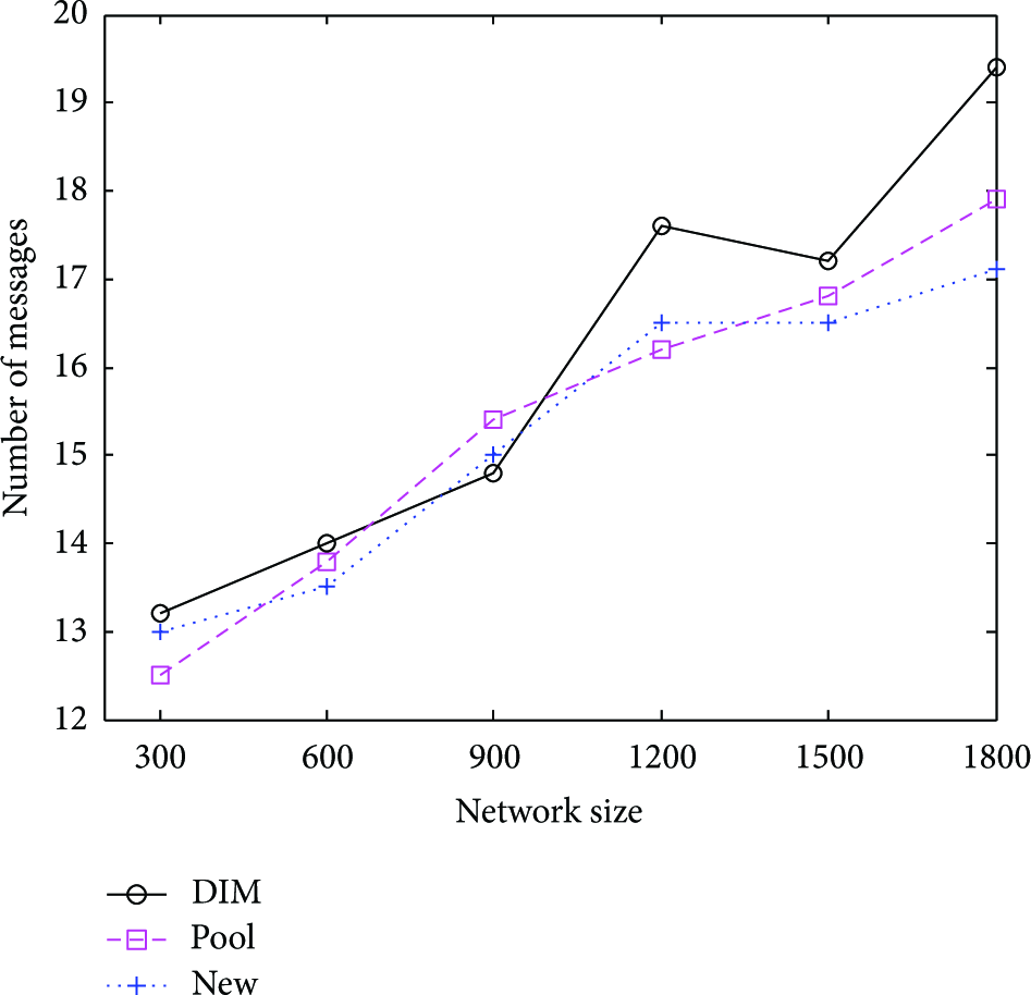
3.2.2. Average Query Delivery Cost

(1) Comparisons on Exact Match Queries

We compared the three algorithms under four different range size distributions and the results are as shown in Figures 3, 4, 5, and 6.

Figure 3

Uniform range size distributions.

Figure 4

Bounded Uniform query size distributions.

Figure 5

Algebraic query size distributions.

Figure 6

Exponential range size distributions.

We can observe some interesting facts from the four figures.

First, all the figures reveal that the range size of a query strongly affects the performance of the three approaches. For instance, all the approaches cost much less in exponential size distribution than in uniform size distribution. This is mainly because data are stored according to splitters like 0.5 and 0.25. The smaller the range size is, the easier a query gets the result. A query therefore has to visit a large amount of storage areas in order to acquire all the answers in uniform size distribution.

Second, the performance result reveals that our algorithm is scalable than Pool, and Pool is scalable than DIM. In DIM all sensors are treated as index nodes. The network needs to construct a huge structure of tree first and that definitely leads to the flood of messages. In Pool the number of pool will not change when the size of network turned larger. A package needs to visit more nodes to get to the destination. In our method the size of the tree is adjustable. We can control the size of flooding area by changing the depth of the tree.

(2) Comparisons on Partial Match Queries

We fixed the size of the network as 900 sensor nodes and compared these methods under one, two, and three of dimensions with specified ranges. The results are as shown in Figure 7 and Figure 8.

Figure 7

Comparisons on partial match dimensions.

Figure 8

Partial match dimension order.

The result in Figure 7 shows that the more dimensions in a query with an unspecified range, the higher the query processing cost would be incurred. The reason is that the more unspecified ranges are, the more index nodes would be accessed which incurs a higher cost. In addition, in the same dimension with unspecified range, DIM costs much more, because it randomly sends the message and the message may route to some unrelated nodes. In one-dimensional partial query, the effect of our method is the same as Pool. The reason is the flooding area becomes large when the number of unspecified range is high. But our method performs better than Pool when the number of unspecified range changed small. The reason is Pool is always searching in the fixed area but ours has changed.

In partial match queries, the location of unspecified dimensions can be changed when its amount is fixed. Figure 8 shows the result of a three-dimensional query.

We can see from Figure 8 that the change of the location of unspecified dimension does not have too much influence to the three methods and Pool is the most stable one. In Pool, the storage area is stable and the number is fixed. The change of the location of unspecified dimension just influences the length from sink to the storage area, but the change in DIM and our scheme can affect the amount and position of the storage area. We can see in Figure 8 that the number of messages is a fluctuating state.

3.2.3. Comparisons on Hot Spot

A good algorithm should have a good mechanism to load balancing. All of the three algorithms have this kind of mechanism. We fixed the size of the network as 900 sensor nodes. Every node sends three packages and the threshold is 20 packages. The result is shown in Figure 9.

Figure 9

Comparisons of hot spot.

We can find that DIM performs worse than Pool, and Pool performs worse than our scheme. In scheme, every node chose a backup node. When it reaches the threshold, the backup node starts to replace it and store data. An event is corresponding to a range and a range is corresponding to a node. So an event directly figures a storage node. In this case, the storage node will soon reach the threshold. In Pool, the storage area is determined by both the events' greatest and the second greatest attribute values. This in some extent divides the similar high-dimensional events again and ensures the storage nodes do not grow too fast. In our scheme, storage area relies on the binary string of the events. The storage node is chosen from the direction of event and it is closest to the center of the storage area. The similar high-dimensional events coming from different directions may store at different nodes. This is the mechanism to load balancing in our scheme. Figure 9 also shows that this method can indeed slow down the production of the number of hot spots.

4. Summary

Data storage and query is an important aspect of data management in WSN. A good storage scheme can give the convenience for the query, save the energy for the network, and greatly extend the network lifetime. For the emergence of multidimensional events, scholars have proposed some ways to ensure the effectiveness of energy. The data storage scheme in this paper is inspired by K-D tree. It first calculates the storage area by encoding the events, then it routes the package to there. The selection of the storage node is related to the direction of the event. In a storage area, there can be different storage nodes and this in some extent ensures the load balancing in the network. The scheme supports multidimensional query through resolving, encoding, and combing the query. In addition, for the integrity of the algorithm the scheme has robustness to package loss and node failure. Finally, we made experiment on the platform of Matlab. The result shows the scheme has much advantage than DIM and is slightly better than Pool, but the complexity and robustness of the scheme are better than both of them.