A Departure Time Choice for Morning Commute Considering Train Capacity of a Rail Transit Line

Abstract

Every commuter utilizing urban rail transit decides the departure time from home to a station according to individual judgment for the biggest possibility to board a train as soon as possible after the arrival. Therefore, the departure time choice behavior of the commuters is complicated especially when the transport capacity of this transit line cannot meet the travel demands of its users in rush hour. This research first develops a travel cost function mainly considering the travel time to rationally describe the volume distribution of the commuters arriving at a station at different time periods. Furthermore, an optimization model is accordingly proposed to rationalize the arrival distribution of the commuters on the basis of the amount of the arrived commuters who are able to board a train from the perspective of the systematic operation of a rail transit line for the minimal total travel cost of all the commuters along this line. It is found that the total travel cost can be reduced by 19.0% at most through the arrival distribution rationalization with the optimization model.

1. Introduction

The growing traffic congestion in large cities has forced traffic to be inefficient and caused high energy consumption. It is generally recognized that the mitigation of these problems requires efficient construction and management of mass transit. However, there are some differences between mass transit and road transport which should be considered. An additional vehicle on a given road generally slows down the speed at which all other vehicles are being driven, causing a time loss to all other drivers; however, an additional commuter on a given train will generally increase the crowding, with no effect on the speed. Many scholars studied the morning commute with different strategic points. The early studies always focused on the principle of the departure time choice of the morning commute such as the equilibrium existence and uniqueness [1–5]. The equilibrium problem is related to many different problems in operations research, such as travel competition [6], heterogeneity of commuters [7, 8], and passenger assignment problem [9].

Reviews discussed the public transport values of time, the delay costs and value of time in trip chains, the behavior and characteristics, and the willingness to pay for travel time reliability of different travelers [10–14]. In the literature, the problem of choosing departure time and route simultaneously in a mass transit system has been studied without explicitly considering capacity constraints. However, many urban mass transits of metropolises have been overloading during morning commute time.

With the bottleneck model widely used in road traffic, early and late penalties were incorporated in the cost function by calculating unit values of early and late arrival times [15–17]. As subway system capacity is limited, too many people traveling in a short period could lead to a waiting time increase or even large scale congregation phenomenon which may be a hazard [18, 19]. The above studies considered crowding as an important influence factor of comfort level and ignored the fact that if the number of commuters waiting at a transit stop exceeds the number of vacant seats on the forthcoming transit run, then some commuters will have to wait for the next run. However, the phenomena in such large cities as Beijing, Hong Kong, London, and New York which appear during peak period, some commuters continue to board the trains even though they have to stand in seriously crowded vehicles. Even more serious, the actual fact that commuters have to wait at platforms for several scheduled intervals caused by larger passenger flow volume in the morning commute has not been described clearly in the past reviews. In Beijing urban mass transit system, for example, scheduled intervals of different lines have been shortened by 28 times in order to increase the transport capacity of the system during the past six years. The daily passenger flow volume of Line 10 of Beijing urban mass transit is currently almost 1.7 million. In a peak period, commuters have to wait for four more trains at some major stations, which may cause them to change their departure time.

In this paper, we focus on the commuters' departure time choice model of the peak period commuting in a mass transit line with multiple origins and a single destination, which may emerge when the mass transit line serves a concentric city where all commuters are assumed to work in a highly compact city centre and live in the dispersed surrounding suburban area. Supposing all commuters are homogeneous with the same work-start time and value of time, the model is intended to describe the general departure pattern of commuters living at various locations traveling to a single destination and how their home locations influence their departure time choices.

This paper is organized as follows. Section 2 introduces the problems and the mathematical expression of the model. We analyze the properties of the model in Section 3. In Section 4, three numerical examples are presented for the model. Section 5 summarizes the paper.

2. Modeling

We consider a mass transit line with multiple origins and a single destination. A train departs from the most distant residential location H₁ and stops by H₂, …, H _K home locations or stations in order of decreasing distance to the workplace W. Suppose that in a morning peak period there are X₁, X₂, …, X _K commuters, who use the transit line from station H₁, H₂, …, H _K to workplace W, respectively. As we consider a daily commuting situation, we assume that the moving time between each line segment from H _K to W (including stopping time at each station) is constant which is denoted by τ₁, τ₂, …, τ _K . Let Z = {ξ, …, 2, 1, 0, −1, −2, …, – ζ} be the tab set of train arrivals at the workplace, where ξ and ζ are sufficiently large to ensure that all commuters can arrive at the workplace during the peak period considered. We can assume that only one train arrives at the workplace W closest to target time h _t , and this train is denoted by 0. Let Λ be the scheduled interval of the line we study which is constant.

For analytical tractability, we assume some conditions as follows.

• Assume that the commuters have sufficient psychological endurance of crowdedness during peak period. Thus, the crowdedness only affects waiting time when there are too many commuters to fit into one train.

• Assume that the urban mass transit is the only option for all commuters in order to find the departure time choice mechanism in one autonomous traffic system.

• Assume that the interval of the line is constant; thus, the supply capacity should be constant also. With only the distribution of arriving commuters in the front stations and knowledge of train supply capacity, we can estimate whether a delay will be caused and calculate the delay further on. If there are too many commuters to catch the trains at upstream stations, the commuters at downstream stations have to depart earlier in order to avoid the late penalty, which will bring the morning peak forward.

2.1. The Total Travel Cost C _i ^j

The generalized travel cost of a path p is a weighted function of ticket price, in-vehicle time, waiting time, walking distance, departure delays, early arrival, number of transfers, and so forth. And we will consider a classical function for the generalized cost, which is the weighted sum of the trip time, the waiting time, and lateness/earliness with respect to the target time. The target time at the destination means that a commuter does not want to arrive later than that time. We will assume that the demand is known; that is, the number of commuters for each O/D pair is given.

The total travel cost of a commuter at station H _i boarding train j is given by

$C_i^j=\alpha ·T_w+\beta ·T_v+\delta \left(h_d\right),$

(1)

where T _w is the waiting time at the platform of the origin station H _i , T _v is the in-vehicle time, and α and β are unit time values of the waiting time and in-vehicle time separately. δ(h _d ) is the early/late arrival penalty when the departure time of the commuter is h _d , whose definition is in line with that in Vickrey's bottleneck model [20].

We assume that this cost has the following three components:

• the time value of waiting time α, which should be bigger than the in-vehicle time value β for commuters feeling anxious;

• the total waiting time T _w spent on the platform waiting for the trains;

• the time that the commuter arrives at the platform of his or her origin station H _i which is denoted as h _d , and h _a is the time he or she reaches destination W. Assuming that commuters have enough information of the mass transit system timetable and they arrive at the platform at the time that a train is arriving, we can get the relationship between h _d and h _a as follows:

  $h_a=h_d+T_w+T_v,$

  (2)

where T _w = nΛ, n is the number of trains large enough to service everyone, and T _v = τ _K .

We can get that

$h_a-h_d=T_w+T_v=n·\mathrm{\Lambda }+{\tau }_K.$

(3)

By definition, h _t is a special case of h _a , so we can get that

$\left|h_t-h_a\right|=j·\mathrm{\Lambda }.$

(4)

Thus, the early/late arrival penalty is given by

$\delta \left(h_d\right)=\delta \left(j\right)=\{\begin{array}{cc}\eta j\mathrm{\Lambda },\hfill & h_a<h_t,\hfill \\ \mathrm{0},\hfill & h_a=h_t,\hfill \\ -\gamma j\mathrm{\Lambda },\hfill & h_a>h_t,\hfill \end{array}$

(5)

where h _t is the target time for each commuter.

2.2. The Number of Commuters Boarding the Train Q _i ^j

If the number of commuters at the platform of station H _i is bigger or equal to the train capacity when train j arrives at station H _i , there must be someone who cannot board the train j as soon as possible after the arrival and has to wait for the train j + 1, so the number of commuters boarding the train j should be the train capacity. On the contrary, if the train capacity is bigger, all the commuters at station H _i could catch this train, so the number of commuters boarding the train j should be equal to the number of commuters at the platform at this moment. The number of commuters boarding the train j at station H _i is given by

$Q_i^j=\min \left(X_i^j,C_i^j\right),$

(6)

where X _i ^j is the number of commuters at the platform of station H _i and C _i ^j is the capacity of the train j when it arrives at station H _i , which is given by

$C_i^j=C^j-{{\displaystyle \sum }}_{k=\mathrm{1}}^{i-\mathrm{1}}{Q}_i^k,$

(7)

specially, when i = 1, C₁ ^j = C ^j .

2.3. The Equilibrium State

Suppose that all commuters attempt to minimize their individual total travel costs by changing their departure times. At equilibrium state, all the commuters departing from the same station have identical total travel cost, and thus no one has an incentive to alter his or her departure time. The desired arrival time at the destination is reflected through formulating the schedule delay penalty. The time of arrival at the station is bound by the choice of arrival trains. With a given transit timetable, the equilibrium commuter departure time distribution $\mathbf{x}=\{x_i^j\mid i=\mathrm{1},\mathrm{2},\dots ,K,j\in Z\}$ can be obtained by solving the following minimization problem:

$\min \mathrm{\hspace{0.17em}\hspace{0.17em}}L\left(\mathbf{x}\right)={{\displaystyle \sum }}_{j\in Z}{{\displaystyle \sum }}_{i=\mathrm{1}}^K\left(\alpha ·T_w+\beta ·T_v\right)+{{\displaystyle \sum }}_{j\in Z}\left({{\displaystyle \sum }}_{i=\mathrm{1}}^K{Q}_i^j\right)\delta \left(h_d\right),\text{subject}\mathrm{\hspace{0.17em}\hspace{0.17em}}\text{to}\phantom{\dots }{{\displaystyle \sum }}_{j\in Z}{X}_i^j=X_i,\phantom{\dots \dots \dots \dots \dots ..}{X}_i^j\ge \mathrm{0}.$

(8)

3. The Model Property

The waiting and schedule delay cost for taking train j at station H _i could be given by

${\lambda }_i^j=\alpha ·T_w+\delta \left(h_d\right)=\alpha ·n·\mathrm{\Lambda }+\delta \left(j\right)=\{\begin{array}{cc}\alpha n\mathrm{\Lambda }+\eta j\mathrm{\Lambda },\hfill & h_a<h_t\hfill \\ \alpha n\mathrm{\Lambda },\hfill & h_a=h_t\hfill \\ \alpha n\mathrm{\Lambda }-\gamma j\mathrm{\Lambda },\hfill & h_a>h_t,\hfill \end{array}$

(9)

where λ _i is the Lagrange multiplier associated with subject (7). For equilibrium conditions, we have

$\begin{array}{c}{\lambda }_i^j\ge {\lambda }_i\hspace{1em}\text{if}\mathrm{\hspace{0.17em}\hspace{0.17em}}{Q}_i^j>\mathrm{0},\\ {\lambda }_i^j>{\lambda }_i\hspace{1em}\text{if}\mathrm{\hspace{0.17em}\hspace{0.17em}}{Q}_i^j=\mathrm{0}.\end{array}$

(10)

The waiting time at station H _i is influenced by both the arriving number of commuters at H _i and the capacity of the train, which is affected by the traffic volume situation of upstream stations.

Theorem 1. At equilibrium, for all j ∈ Z, 1 < i ≤ K, if Q _i ^j > 0, then ${\sum }_{k=\mathrm{1}}^{i-\mathrm{1}}{Q}_k^j>\mathrm{0}$ .

Proof. We provide a proof of the theorem by contradiction. Suppose there exists station i and train j such that Q _i ^j > 0 and ${\sum }_{k=\mathrm{1}}^{i-\mathrm{1}}{Q}_k^j=\mathrm{0}$ , which means that X _k ^j = 0 or C _k ^j = 0 at each station's upstream station i.

For k = 1, 2, …, i – 1, if C _k ^j = 0, the train j must have been full, so Q _i ^j = 0 which violates the known condition Q _i ^j > 0; if X _k ^j = 0, j may not be in the set Z.

Thus, there exists no i and j such that Q _i ^j > 0 and ${\sum }_{k=\mathrm{1}}^{i-\mathrm{1}}{Q}_k^j=\mathrm{0}$ .

Theorem 1 proposed that if a train is chosen by commuters at a nonstarting station at the equilibrium of commuting during the peak period, this train must have also been chosen by commuters from upstream station or stations. Consequently, commuters at an intermediate boarding station must ride a train together with the commuters from some stations further upstream.

Theorem 2. At equilibrium, for any given X _i ^j , there is no commuter choice in the departure time for train ξ or – ζ.

Proof. If a commuter can depart at time ξ – Δt (Δt > 0) in order to reduce his or her total travel cost, this situation is incompatible with the definition of equilibrium. Thus, X _i ^ξ = 0. Similarly, we can prove that X _i ^−ζ = 0.

Theorem 2 proposed that there is no commuter choice in the earliest or latest departure times at equilibrium.

Theorem 3. At equilibrium, for all j ∈ Z, 1 < i ≤ K, if Q _i ^j = C _i ^j = 0, then ${\sum }_{k=i+\mathrm{1}}^K{Q}_k^j=\mathrm{0}$ .

Proof. When Q _i ^j = C _i ^j = 0, this train has been full at the upstream stations of H _i ; thus no commuters at the stations downstream of H _i can catch the train j.

Theorem 3 proposed that the commuters at the upstream stations of the line can get to the workplace W at a time near the target time h _t ; however, the commuters at the downstream stations have to choose a departure time far away from the target time and get to the workplace early or late if the total number of commuters is too big to transport. A limit should be imposed on commuters boarding a train for security reasons. For example, the peak period number of commuters on the upstream station in Beijing is limited by metro staff in order to reduce the load factor with a busy line.

4. Numerical Examples

To illustrate the application of the proposed model and solution algorithm, a simple numerical example is presented in this section. Given sufficiently large ξ and ζ, the equilibrium solution can be obtained numerically. We provide a simple example with three origins and a single destination as shown in Figure 1.

Figure 1:

Distribution of commuter departures for a mass transit line with four stations.

The parameters are as follows: K = 3, (α, β, η, γ) = (10, 0.5, 0.1, 10.0) RMB/h, Λ = 0.05 h, C = 180,(τ₁, τ₂, τ₃) = (0.2, 0.1, 0.2) h, and (X₁, X₂, X₃) = (1600, 1400, 1200). We solve the integral number planning of mathematical programs example directly by a standard YALMIP function of MATLAB. Figure 2 plots the distribution of commuter departures at equilibrium at each station.

Figure 2:

Distribution of commuter departures with three stations when (α, β, η, γ) = (1.0, 0.5, .1, 10.0).

Figure 2 shows the solution obtained by solving the resultant system of equations. It is observed that the set consists of train services that were utilized (j = 23, 22, …, 1, 0) during the peak-period. There is no commuter arriving at the workplace after the target time since the late penalty is much larger than the early penalty. At the beginning of the peak period, the commuters at the three stations choose the different trains shown in the figure.

The commuters who arrive at the workplace near the target time come from station 1, located at the beginning of the line. The capacity constraint of the train makes it impossible for commuters at other stations to board the train unless there are some measures enforced to ensure that the capacity of forthcoming trains is large enough.

4.1. The Uncertainty Analysis of the Early/Late Penalty

We analyze the mechanism of how the early/late penalty influences departure time choice by the commuters in different stations through the following uncertainty analysis. For a convenient comparison, we only change the values of η and γ.

Figures 3 and 4 plot the distributions of commuter departures at equilibrium when the values of time parameters are (η, γ) = (1.0, 10.0) RMB/h and (η, γ) = (10.0, 10.0) RMB/h, respectively.

Figure 3:

Distribution of commuter departures with three stations when (α, β, η, γ) = (1.0, 0.5, 1.0, 10.0).

Figure 4:

Distribution of commuter departures with three stations when (α, β, η, γ) = (1.0, 0.5, 10.0, 10.0).

As shown in Figure 3, there exist some commuters who arrive at the workplace after the target time which is different from Figure 2. The set consists of train services that were utilized (j = 21, 20, …, 1, 0, −1, −2) when the early penalty is one-tenth of the late penalty. Late commuters who arrive at the station W increased.

Figure 4 shows that the set consists of train services that are utilized (j = 12, 11, …, 1, 0, −1, …, −11) when the early penalty is equal to the late penalty.

4.2. With a Limit Outside the Stations

The results of the examples above show that a train was fully occupied at the first station because commuters in the same station will go together. To better fit reality, we assume that there is a limit outside the station which is defined by Φ. In this example, we use K = 3, (α, β, η, γ) = (1.0, 0.5, 0.1, 10.0) RMB/h, Λ = 0.05 h, C = 180,(τ₁, τ₂, τ₃) = (0.2, 0.1, 0.2) h, (X₁, X₂, X₃) = (1600, 1400, 1200), and Φ = 80. Figure 5 plots the distribution of commuter departures at equilibrium with a limit outside the stations.

Figure 5:

Distribution of commuter departures with a limit outside the stations when (α, β, η, γ) = (1.0, 0.5, 0.1, 10.0).

Figure 5 shows that the set consists of train services that utilized (j = 22, 21, …, 1, 0) during the peak period. The commuters farther away from the workplace will always ride the trains with arrival times closest to work-start time until a limit is reached due to train capacity or outside regulation. Thus, some commuters choose the trains near the target time rather than choose a train far away from target time in order to reduce the total travel cost.

Again, we assume that there is a limit outside the station which is defined by Φ. In this example, we use K = 3, (α, β, η, γ) = (1.0, 0.5, 1.0, 10.0) RMB/h, Λ = 0.05 h, C = 180, (τ₁, τ₂, τ₃) = (0.2, 0.1, 0.2) h, (X₁, X₂, X₃) = (1600, 1400, 1200), and Φ = 80. Figure 6 plots the distribution of commuter departures at equilibrium with a limit outside the stations.

Figure 6:

Distribution of commuter departures with a limit outside the stations when (α, β, η, γ) = (1.0, 0.5, 1.0, 10.0).

Figure 6 shows that the set consists of train services that were utilized (j = 21, 20, …, 1, 0, −1) during the peak period. The distribution of commuter departures at equilibrium is almost the same as Figure 5 except for the trains arriving later than the target time.

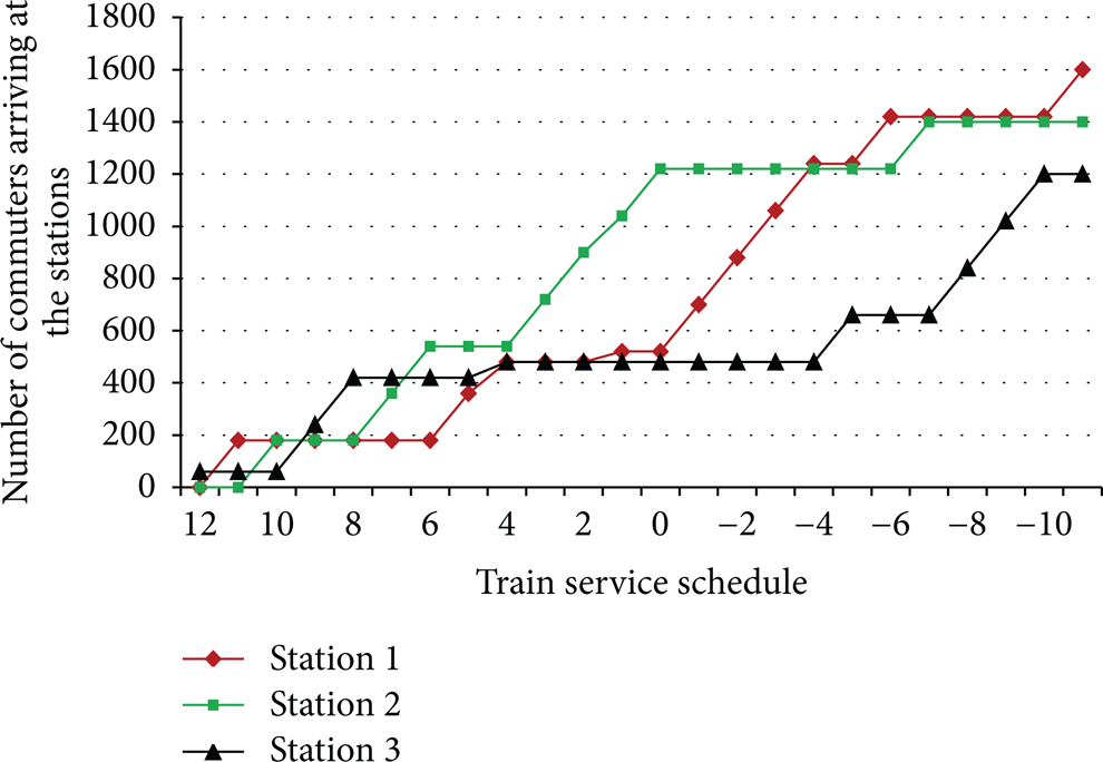
We assume once again that there is a limit outside the station which is defined by Φ. In this example, we use K = 3, (α, β, η, γ) = (1.0, 0.5, 10.0, 10.0) RMB/h, Λ = 0.05 h, C = 180, (τ₁, τ₂, τ₃) = (0.2, 0.1, 0.2) h, (X₁, X₂, X₃) = (1600, 1400, 1200), and Φ = 80. Figure 7 plots the distribution of commuter departures at equilibrium with a limit outside the stations.

Figure 7:

Distribution of commuter departures with a limit outside the stations when (α, β, η, γ) = (1.0, 0.5, 10.0, 10.0).

Figure 7 shows that the set consists of train services that utilized (j = 12, 11, …, 1, 0, −1, …, −10) during the peak period when the early penalty is equal to the late penalty. The distribution of commuters is a normal distribution and the intermediate point is the train that arrives at the workplace at the target time.

4.3. The Optimization Results Analysis

The volume distribution of commuters arriving at a station at different time periods of morning rush hour is assumed as a Poisson distribution [21–23].

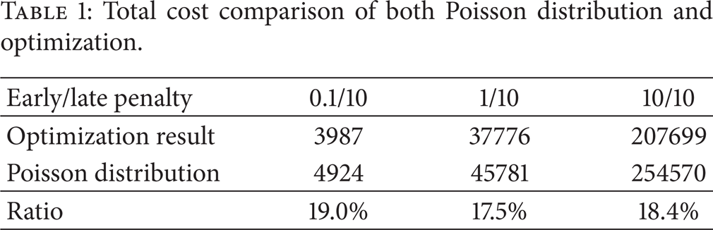
The total costs in three scenarios have been reduced by 17.5%–19.0% through the arrival distribution rationalization optimization, which are shown in Table 1.

Table 1:

Total cost comparison of both Poisson distribution and optimization.

Early/late penalty	0.1/10	1/10	10/10
Optimization result	3987	37776	207699
Poisson distribution	4924	45781	254570
Ratio	19.0%	17.5%	18.4%

5. Conclusions

In this study, a travel cost function mainly considering the travel time to rationally describe the volume distribution of the commuters arriving at a station along a rail transit line with multiple origins and a single destination has been proposed. Constraints of the train capacity in departure time choice but not the crowding cost are considered which are based on the current state of the Beijing mass transit system. An optimization model is accordingly proposed to rationalize the arrival distribution of the commuters on the basis of the amount of the arriving commuters who are able to board a train from the perspective of the systematic operation of a rail transit line for the minimal total travel cost of all the commuters along this line. We clearly show the following general properties of the equilibrium departure time distribution of commuters at equilibrium.

1. The analytical and numerical results show that the commuters living nearer to the workplace will not ride the train together with the commuters living farther away from the workplace until there is an external limit imposed.

2. The commuters farther away from the workplace have more freedom to choose, and the commuters closer to the workplace have to take the earlier and later trains in order to avoid the fully loaded train that cannot service them.

3. At each station, there is a set of train services during the peak period that utilizes a maximum constant number of commuters for each train.

It is found that the total travel cost can be reduced by 19.0% at most through the arrival distribution rationalization with the optimization model. As a result, it is suggested that the information about the amount of people at each station of a rail transit line particularly in rush hour should be released by operating company in order to make arrival distribution optimal. Further work will be devoted to consider the variable train service frequency for generality and the heterogeneity of the commuters on the target time or value of time.

Conflict of Interests

The authors declare that they have no competing financial interests.