Sage Journals: Discover world-class research

Abstract

Data aggregation scheduling in ubiquitous sensor networks is a major research interest for many researchers. Very little research is carried out to schedule the nodes in ubiquitous sensor networks for maximizing the throughput and utilize the hardware resources effectively. The traditional graph model does not model the interferences occurring from the concurrent transmissions in the Ubiquitous Sensor Networks. Hence in this paper we propose a new network model for the USN called a power control collision interference free model and a novel distributed data aggregation scheduling protocol which is adaptive to the rate and power. We tested the protocol in a USN consisting of 50, 100, 150, 200, and 250 number of nodes with different topologies and varying degree 2, 4, 6, 8, 10, 12, 14, 16, 18, 20, …, 40. We compared our results with the other protocols and proved that our proposed power control collision interference free model yields better results.

1. Introduction

RFID (radio frequency identification) is a technology which is used to acquire information anytime and anywhere through network access service [1]. Such ubiquitous network yields better results when integrated with wireless sensor networks (WSNs). This integrated network is called a ubiquitous sensor network (USN) [2]. Several servers participate in ubiquitous networks and the flow of data across the network is as follows (1)

the sensors detect events,

(2)

the RFID readers recognize tags,

(3)

the information is forwarded to one or more servers,

(4)

depending on the arrived event, the servers integrate data from RFID networks and WSNs fire the necessary procedures,

(5)

each intermediate sensor implements method for data aggregation and filtering.

Generally the following are some of the limitations of RFID networks when integrated with WSN: (1)

all the nodes share a single wireless channel for transmission and when multiple nodes transmit at the same time, their transmission may get collided,

(2)

nodes cannot receive and send simultaneously since they are equipped with a single half-duplex radio transceiver [3],

(3)

bandwidth and battery power are the two resource limitations for RFID active tags and sensors,

(4)

retransmissions after collisions, overhearing and overemitting reduce the efficiency of USN.

Hence in order to overcome such limitations, an efficient schedule for data aggregation is needed. Each ubiquitous node in USN should forward data to the base station. Each node does not forward data to the base station directly. Instead it forwards data to a special node called head node. The head node in turn forwards data to the base station. Each node obtains a frequency for transmitting in one or more time slots.

The following are the two main objectives of our paper: (1)

selection of the head node,

(2)

finding a schedule which decides the following:

(a)

when head nodes should transmit,

(b)

how the head nodes gather data from their neighbors.

Since the ubiquitous nodes change their state dynamically, finding a solution to the above mentioned tasks is very difficult.

An optimal schedule is a schedule with (a)

minimum number of time slots (frame length),

(b)

maximum number of concurrent transmissions per each time slot.

USNs are commonly modeled using (1)

traditional graph model,

(2)

physical interference model.

The traditional graph model does not model the interferences occurring from the concurrent transmissions.

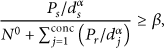
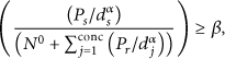
In the physical interference model, the transmission becomes successful if and only if the signal-to-interference-noise-ratio (SINR) perceived at the receiver is above a certain threshold.

For example, if $V_{j}$ denotes a node that can transmit concurrently with node $V_{i}$ as the head, then for a successful transmission the SINR perceived at the receiver should be greater than or equal to β.

That is,

\begin{matrix} \frac{P_{s} / d_{s}^{α}}{N^{0} + \sum_{j = 1}^{conc} (P_{r} / d_{j}^{α})} \geq β, \end{matrix}

(1)

where

(a)

$P_{s}$ and $P_{r}$ are the transmission powers of sender and receiver nodes,

(b)

$d_{s}$ is the distance between the sender and receiver nodes,

(c)

$d_{j}$ is the distance between a concurrent transmitter and the receiver nodes,

(d)

α is the path loss ratio which has a typical value between 2 and 4,

(e)

$N^{0}$ is the ambient noise, and

(f)

β is the threshold for a successful transmission.

Earlier several centralized and distributed scheduling algorithms are proposed for data aggregation in USN [4, 5]. In this paper, we presented a novel distributed data aggregation scheduling protocol using a power control collision-interference-free model. Our proposed protocol is adaptive to the rate and power control and also yields better results when compared with the other existing protocols.

2. The Proposed Power Control Collision Interference Free Ubiquitous Sensor Network Model

Consider a ubiquitous sensor network with n arbitrarily distributed ubiquitous nodes. Let a directed graph $G = (V, E)$ denote a ubiquitous network, where $V = {v_{0}, v_{1}, v_{n - 1}}$ and $E = {e_{0}, e_{1}, e_{n - 1}}$ . $V_{i}$ denotes ubiquitous node i, and $e_{i}$ denotes the edge between two ubiquitous nodes. The minimum Euclidean distance between a pair of nodes is 1. The transmission is assumed to be half duplex.

Each node in the proposed power control collision interference free model is characterized by an 8-variable vector

(
Nodetype	Nodeid
Info	Location
NodeState	State
Integer	number of neighbors
CRange	communication range, Max Crange
IRange	interference range, Max Irange
Power	transmission power, MaxPower
Distance	distance from base station
)

The location denotes the global location of a ubiquitous node. Each node exists in two states called active and inactive states. The nodes that are willing to transmit are said to be in active state and are termed as active nodes, while the remaining nodes are said to be in inactive state and termed as inactive nodes. The state of a node changes frequently.

Now we model a ubiquitous sensor network as USN (V, crmax, ρ), where the following hold. (1)

V is the set of n ubiquitous nodes each characterized with the 8-variable vector.

(2)

crmax is the maximum communication range.

(3)

$ρ \geq 1$ is the interference factor.

(4)

Each node can send and receive data in the maximum range crmax.

(5)

The transmission power of a node is always ≤ crmax.

(6)

Let $V_{j}$ denote a node that can transmit concurrently with node $V_{i}$ as the head. For a successful transmission the SINR perceived at the receiver should be greater than or equal to β; that is,

\begin{matrix} (\frac{(P_{s} / d_{s}^{α})}{(N^{0} + \sum_{j = 1}^{conc} (P_{r} / d_{j}^{α}))}) \geq β . \end{matrix}

(2)

Let

P_{s}

and

P_{r}

denote the transmission powers of sender and receiver nodes respectively,

d_{s}

is the distance between sender and receiver nodes and

d_{j}

is the distance between a concurrent transmitter and the receiver, α is the path loss ratio, which has a typical value between 2 and 4,

N^{0}

is the ambient noise, and β is the threshold for a successful transmission.

(7)

Every node has the flexibility to tune itself to an optimal power.

The spatial reuse and data rates are the two important factors to be considered to improve the efficiency of the USN. As the signal strength decreases with the square of the distance according to the free space path loss model, the interference range is assumed to be two times the required distance between the nodes in order to avoid interferences. Generally larger transmission powers result in high data rates but allow a few concurrent transmitters. Similarly smaller transmission powers result in low data rates but allow more concurrent transmitters. Hence an optimal transmission powers are chosen to improve the overall network capacity.

3. Distributed Algorithm

The models for representing Networks are divided into three categories [6]: (1)

tree based,

(2)

cluster based,

(3)

hybrid topology.

In tree based structure, the root of tree is called sink node. Data flows from leaf nodes to sink nodes through one or more intermediate nodes [6, 7]. These intermediate nodes are called aggregator nodes. Aggregator nodes in turn add their own monitored data and send the aggregated data to its parent node [6].

In clustered approach, every cluster has a cluster head and the entire node in this cluster transmit data to the cluster head (CH). This CH either transmits data to sink node or to the CH of another cluster which is nearest to sink node [6].

In [8] a new adaptive distributed broadcast scheduling method for mobile ad hoc networks is proposed. In [9, 10] a method for maximizing the channel throughput in mobile ad hoc networks using mIDS is proposed. In [11] an ACSP interceptor for improving network capacity in mobile ad hoc networks is proposed.

In this paper we proposed a novel solution for improving the performance of USN. It consists of the following three steps: (1)

identification of ConcHead Nodes,

(2)

constructing a schedule with a list of neighbors of ConcHeads,

(3)

finding an optimal schedule.

The protocol Optimal_SHDL will (1)

identify the ConCHead nodes,

(2)

construct a set of schedules from which an optimal schedule is also founded.

Generally time is slotted to intervals where L denotes the length of the interval.

A schedule is a sequence of time slots. All noninterfereing nodes $u_{i}$ are scheduled to send their aggregated data to any of their neighbors, $v_{i}$ . The power $p_{i}$ chosen at $v_{i}$ cannot exceed the value of the MaxPower. Formally, at each time slot t, we have an assignment vector:

\begin{matrix} {AssignVect}_{k} = ((u_{1}, v_{1}, p_{1}), (u_{2}, v_{2}, p_{2}), \dots, (u_{k}, v_{k}, p_{k})) . \end{matrix}

(3)

Generally if each node knows when to transmit, ideal listening can be avoided. Every node after receiving or transmitting data goes to sleep mode or for processing the data until its next time slot, and this technique saves battery power [6].

Our distributed algorithm is an iterative process and ends when the complexity of the ConCHeadTree cannot be further decreased. The algorithm is as follows.

Algorithm 1.0 PCCIF (UV, N)

UV represents the set of of Ubiquitous nodes

N represents the total number of nodes

Step 1. Construct a PCCIF_Network from the set of nodes UV

Step 2. ConCHeadTree = Tree_traversal (PCCIF_Network, UV, N)

//Construct ConCHead Tree from the PCCIF_Network

Step 3. ConCHeadList = Optimal_SHDL (ConCHeadTree)

//Construction of Optimal Schedule contains three phases where we identify a list of ConCHeadnode, their neighbors, the schedule for transmission and an optimal schedule

Step 4. Empty List UV

Step 5. Set UV = ConCHeadList

//We rebuild a USN with the ConCHeadnode identified and in the new USN, the ConCHeadnode are the normal nodes

Step 6. Find complexity of the new USN

Step 7. If complexity level is above a threshold then

Forward_to_Base(ConcHeadList)

Goto Step 8

Else

Goto Step 1

Step 8. End.

An optimal schedule is constructed with edges from E. The total transmission time T consists of slots ${t_{0}, \dots, t_{T - 1}}$ and the total schedule $S = {S_{0}, S_{1}, \dots, S_{T - 1}}$ , where $S_{t}$ denotes the subset of nodes in V scheduled to transmit in time slot $t_{i}$ .

The optimal schedule satisfies the following conditions: (a)

each active node may be scheduled more than once but must be scheduled at least once,

(b)

a node cannot act as a transmitter and a receiver in the same time slot, in order to avoid the primary interference [12],

(c)

a head node vi transmits to the base station only after all its neighbors have been scheduled [13],

(d)

we use the path loss radio propagation model [14] to characterize path loss:

\begin{matrix} p_{recv} = \frac{p_{trans}}{d^{α}}, \end{matrix}

(4)

where

p_{recv}

and

p_{trans}

are the transmit powers at the receiver and transmitter, d is the distance between the transmitter and the receiver, and α is the path loss exponent, ranging from 2 (line of sight free space) to 4 (indoor).

The construction of an optimal schedule from the proposed power control collision interference free model is as follows.

Given a USN tree, then the procedure Optimal_SHDL (ConCHeadTree) consists of the following phases.

( 1) Head Selection Phase. Construct one or more ConCHeadTrees and from each ConCHeadTree identify one or more ConCHeads.

( 2) Aggregation Scheduling Phase. Construct a schedule with the list of active nodes for each ConCHeadnode. All the neighbors of each ConCHeadnode are assigned different frequencies from the Frequencyset ${f_{1}, f_{2}, f_{3}, f_{4}, \dots, f_{n}}$ . Hence they can transmit to the ConCHeadnode at the same time concurrently in the same slot without any interference.

Let $A V_{i j}$ , for $i, j = 1, \dots, n$ , denote the set of active nodes for each ${ConCHeadnode}_{i}$ . Assign a unique frequency and a time slot in the schedule for each $A V_{i j}$ . These frequencies are allocated in such a way that there are no interferences among the concurrent transmitters and the SINR constraint is satisfied.

The above two steps are iterative and end when all the nodes are termed as either ConCHeadnodes or a neighbor to the ConCHeadnodes. There exists one or more ConCHeadnodes to forward the aggregated data to the base station and each ConCHeadnode has zero, one or more neighbors from where it gathers the data. Generally a ConCHeadnode is selected based on a criterion that improves the utilization of the hardware resources and maximizes the network throughput. The schedule consists of one or more slots. And at the end of the two phases a set of schedules are identified.

( 3) Optimal Scheduling Phase. The optimal schedule is constructed from the schedules constructed in the previous phases. An optimal schedule always improves the network capacity and also best utilizes the hardware resources at each ubiquitous node.

Algorithm 2.0 Optimal_SHDL

Step 1. Let N denote the number of nodes in USN and UV denote the set of all N nodes in USN

Step 2. for $i = 1,2, 3, \dots, N$ do Steps 3 to Steps 6

Step 3. NodeSet = UV, $j = 1$

Step 4. Increment s by 1

Step 5. Repeat until NodeSet = NULL or no new traversal on USN

(5.1) Increment k by 1

(5.2) Empty ConCHeadList

(5.3) ${ConCHeadList [{UV}_{i}], Totalnodes [{UV}_{i, j}]}$ =

Tree_Traversals( ${UV}_{i}, i, j, UV$ )

(5.4) Construct Schedule [s, Slot[k], ConCHeadList [ ${UV}_{i}$ ], totalnodes [ ${UV}_{i, j}$ ]]

(5.5) For each node X in ConCHeadList do

NodeSet = NodeSet − Activeneighbor[X]

(5.6) NodeSet = NodeSet – ConCHeadList

(5.7) Increment j by 1

End

Step 6. If NodeSet ! = NULL then

For Each node X in NodeSet do

Construct Schedule [s, Slot[k], X, 1]

Increment k by 1

End For

Step 7. Call Optimal_traversal (Schedule, s)

Step 8. End.

Algortihm 3.0. Tree-Traversals (A, i, j, NodeSet)

//neighbors A contains 1-hop neighbors list of a node

//non_conflict_set [A] contains the list of nodes that donot produce Type 1 or Type 2 interfernces with A

//Possible_frequency_set.—Contains the frequency with which the node A's neighbors can transmit

//ActiveNeighbor [X] contains list of neighbors who are transmitting alogn with X

(1.0) neighbors $A []$ ← Assign 3-hop, 4-hop $\dots n$ -hop

Neighbors list of A

(2.0) non_conflict_set [A] ← Find from neighbors $A []$ the set of non-conflicting nodes that can transmit along with A.

(3.0) for each node X in non_conflict_set [A] repeat thru steps 4.0 to 8.0.

(4.0) ActiveNeighbor [X] = neighbors [X]

(5.0) Let Possible_ Frequency_set [X] ←

Assign (ActiveNeighbors [X], Frequencyset $[]$ )

(6.0) if ActiveNeighbor [X] is having Type 1 or Type 2 interferences with any 1-hop neighbors of each node in non_conflict-set [A] then

AcitveNeighbor [X] = Poweradaption (ActiveNeighbor, X, non_conflict_set, A)

(7.0) Totalnodes [ $A, j$ ] = Totalnodes [ $A, j$ ] + number of nodes in ActiveNeighbor [X]

(8.0) End For

(9.0) Return non_conflict_set [A], Totalnodes [ $A, j$ ]

(10.0) End.

Algorithm 4.0

PowerAdaption (ActiveNeighbor, X, non_conflict_set, A)

// $Concurren t_{i}$ denotes the list of concurrent nodes transmitting along with node i

Step 1. For each u in ActiveNeighbor [X] do steps 2 thru steps 4

Step 2. AssignLevel = false, conc = ${concurrent}_{u}$

Step 3. For each $P_{s}$ in $P_{low}, \dots, P_{high}$ do

\begin{matrix} (\frac{(P_{s} / d_{s}^{α})}{(N^{0} + \sum_{j = 1}^{conc} (P_{r} / d_{j}^{α}))}) \geq β, \end{matrix}

(5)

then

Assign Power $P_{s}$ to u

Assign Level = true

Break

Step 4. If AssignLevel = false then

ActiveNeighbor [X] = ActiveNeighbor [X] − u

Step 5. Return (ActiveNeighbor)

Step 6. End.

Algorithm 5.0 Optimal_traversal (Schedule, s)

Step 1. For I in s repeat steps 2 thru

Step 2. //To Maximize total number of concurrent transmissions

Construct NewSchedule I after Arranging slots in Schedule I in descending order of the totalnumberofnodes for each slot.

Step 3. //To Minimize frame length

Remove a slot consisting of minimum number of nodes from NewSchedule I if all its nodes appear in other remaining slots in NewSchedule I

Step 4. End For

Step 5. DescSort (NewSchedule, s)

Step 6. OptimalSchedule = NewSchedule [1]

Step 7. End.

4. Results

In [11] the authors assumed a $1000 \times 1000$ square meter rectangular simulating area. The number of nodes in the simulation varied from 2 to 40. They tested with 50 different topologies where each mobile station can tune to its required transmission power. They observed that the average time slots increase linearly as the number of nodes increases for all three algorithms. And they also observed that the Greedy has the smallest schedule length and the RTS/CTS algorithm generates the longest schedule and that the performance difference between these three algorithms is insignificant for small network sizes (less than 17 nodes) and is larger when the network becomes large.

In this paper we assumed the same simulating parameters and we obtained the number of time slots from the PCCFI as 4, 8, 10, 12, 15, 17, and 18 when N = 10, 15, 20, 25, 30, 35, and 40, respectively. These results are shown in Figure 1. From [11] we observed that the numbers of time slots of the Greedy, RTS/CTS, and Ranked Schedule methods are far less than 4, 8, 10, 12, 15, 17, and 18 when N = 10, 15, 20, 25, 30, 35, and 40, respectively. Hence these results convey that the PCCFI method outperforms nearly 30–50% of the existing Greedy, Ranked Schedule, and RTS/CTS methods.

Figure 1

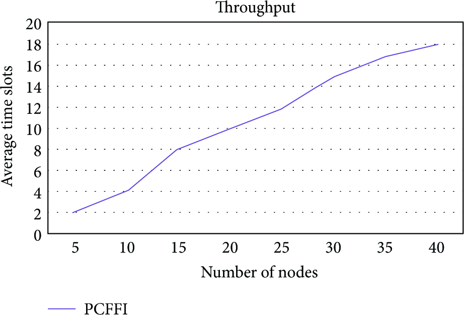
Throughput from PCCFI Simulating area $1000 \times 1000$ square meter rectangular area, where $N = 5,10,15, \dots, 40$ .

In [15] the authors assumed a 200-square area, with 25 m of transmission range. The SDA [16], PAS [17], DAS [18], SAS [19] and First-Fit [20] algorithms are executed with different densities and the results for an average of 10 runs are reported. They compared these algorithms performance with WIRES-BSPT [15]. Since First-Fit algorithm does not produce a conflict free schedule, it is omitted from the evaluations. They concluded that WIRESBSPT [15] outperforms all other solutions by 10% to 30%.

In this paper we assumed the same simulating parameters and with different datasets. The results are shown in Figure 2. These results show that the maximum time slots required by the proposed method are 10, 18, 28, 45, and 65 when N = 20, 40, 60, 80, and 100, respectively.

Figure 2

Throughput from PCCFI Simulating area 200 square area, where $N = 20,40, \dots, 100$ .

The maximum time slots required by SDA [16], PAS [17], DAS [18], SAS [19], WIRES-BSPT [15], and First-Fit [20] are less than 10, 18, 28, 45, and 65 when N = 20, 40, 60, 80, and 100, respectively. Hence our proposed PCCFI method outperforms the SDA [16], PAS [17], DAS [18], SAS [19], WIRES-BSPT [15], and First Fit methods by 30–50%.

Hence our proposed algorithm outperforms the results obtained from Greedy, RTS/CTS, Ranked Schedule, SDA, PAS, DAS, SAS, WIRES-BSPT, and First Fit by 30–50%.

5. Conclusion

In this paper we proposed a new network model for the USN called power control collision interference free model. We also presented a distributed data aggregation scheduling protocol using the proposed model which is adaptive to the rate and power for USN.

Generally there is a high correlation between the transmission power of a node, number of concurrent transmitters and their spatial distances. Larger transmission powers results high data rates but allow a few concurrent transmitters. Similarly smaller transmission powers results low data rates but allow more concurrent transmitters. Therefore, the transmission powers are adjusted according to the number of concurrent transmitters and their distances to yield a maximum network capacity.

References

Park

Gadh

Kim

Won

System framework and its application in mobile RFID Service network

Selected Topics in Communication Networks and Distributed Systems 2010 113

Lee

H.-C.

Hwang

J.-H.

Yoe

Energy efficient MAC protocol for ubiquitous agriculture

International Journal of Smart Home 2010 4 3 15

Liao

W. H.

Shih

K. P.

Chung

W. C.

Multi-channel medium access control protocol with channel distribution for mobile ad hoc networks

Communications IET 2009 3 12 1821 1831

10.1049/iet-com.2008.0692

Sharad Mishra

Sharma

A. K.

Chauhan

D. S.

Analysis on energy optimized data collection in tree based ad-hoc sensor network

International Journal of Modern Education and Computer Science 2012 42 49

Wan

P. J.

Alzoubi

K. M.

Frieder

Distributed construction of connected dominating set in wireless ad hoc networks

Mobile Networks and Applications 2004 9 2 141 149

Kumar

Chauhan

A survey on scheduling algorithms for wireless sensor networks

International Journal of Computer Applications 2011 20 5, article 2

Kim

Park

Chong

P. K.

Sung

Kim

Distributed low power scheduling in wireless sensor networks

Proceedings of the 2nd International Symposium on Wireless Pervasive Computing (ISWPC ′07)

February 2007

San Juan, Puerto Rico, USA

268 273

2-s2.0-34548127855

10.1109/ISWPC.2007.342613

Madhavi

A new adaptive distributed broadcast scheduling method for mobile AdHoc networks

Proceedings of the 4th International Conference IEEE Digital Xplore, Networking and Services (ICNS ′08)

March 2008

7978 7120

Madhavi

RameshBabu

Maximizing the channel throu-ghput in mobile adhoc networks using mIDS

International Journal of Wireless Communications Issue September 2009

10.

Madhavi

RameshBabu

An ACSP interceptor for improving network capacity in mobile adhoc networks

Masaum Journal of Computing 2009 1 3 382 388

11.

Choi

Wang

Hughes

E. A.

Scheduling for information gathering on sensor network in Wireless Networks

Wireless Networks 2009 15 1 127 140

12.

Sheikhpour

Jabbehdari

Zadeh

A. K.

A cluster-chain based routing protocol for balancing energy consumption in wireless sensor networks

International Journal of Multimedia and Ubiquitous Engineering 2012 7 2

13.

Tripathy

A. K.

Chinara

Comparison of residual energy-based clustering algorithms for wireless sensor network

ISRN Sensor Networks 2012 2012 10

375026

10.5402/2012/375026

14.

Kim

Lim

Hou

J. C.

Improving spatial reuse through tuning transmit power, carrier sense threshold and data rate in multihop wireless networks

Proceedings of the 12th annual international conference on Mobile computing and networking (MobiCom ’06)

September 2006

Los Angeles, Calif, USA

ACM

366 377

15.

Malhotra

Nikolaidis

Nascimento

M. A.

Aggregation convergecast scheduling in wireless sensor networks

Wireless Networks 2011 17 2 319 335

2-s2.0-79951517873

10.1007/s11276-010-0282-y

16.

Chen

Zhu

Minimum data aggregation time problem in wireless sensor networks

Lecture Notes in Computer Sciences 2005 3794 133 142

17.

Mehrotra

Venkatasubramanian

Sensor scheduling for aggregate monitoring in wireless sensor networks

Proceedings of the 19th International Conference on Scientific and Statistical Database Management (SSDBM ′07)

2007

18.

Distributed data aggregation scheduling in wireless sensor networks

Proceedings of the 28th Conferenceon Computer Communications (INFOCOM ′09)

Rio de Janeiro, Brazil

2159 2167

19.

Wan

P. J.

Huang

S. C. H.

Wang

Wan

Jia

Minimum latency aggregation scheduling in multihop wireless networks

Proceedings of the 10th ACM International Symposium on Mobile Ad Hoc Networking and Computing (MOBIHOC ′09)

185 194

20.

Huang

S. C. H.

Wan

P. J.

C. T.

Yao

Nearly constant approximation for data aggregation scheduling in wireless sensor networks

Proceedings of the 26th Conference on Computer Communications (INFOCOM ′07)

366 372

A Dynamic and Distributed Scheduling for Data Aggregation in Ubiquitous Sensor Networks Using Power Control

Abstract

1. Introduction

2. The Proposed Power Control Collision Interference Free Ubiquitous Sensor Network Model

3. Distributed Algorithm

4. Results

5. Conclusion

References