Sage Journals: Discover world-class research

Abstract

A methodology is proposed to apply an endurance function model with a genetic algorithm to estimate the fatigue life of notched or smooth components. The endurance function model is based on stress tensor invariants and deviatoric stress invariants. In the proposed methodology, FEA is used to simplify the application of the endurance function model. Experimental results from published literature are considered for the case studies to evaluate the proposed methodology. The results show that the proposed methodology simplified the application of the endurance function model, particularly by reducing the need for notch sensitivity factors, and the stress invariants can be calculated directly from the stresses at the critical point. The comparison with experimental results shows that, with proper calibration, the model can predict fatigue life accurately.

1. Introduction

Since the investigations by Wohler in 1860, fatigue experiments and predictions have played a major role in mechanical design [1, 2], and researchers investigating the fatigue problem have made huge efforts in order to devise sound methodologies suitable for safely assessing mechanical components subjected to time-variable loadings [3 –7]. It is acknowledged globally that correctly estimating fatigue damage in real components is a complex process involving a high number of different variables that have to be properly taken into account in order to avoid unwanted and dangerous failures [8]. Any reliable fatigue assessment technique should be able to efficiently and simultaneously model the damaging effect of nonzero superimposed static stresses, the degree of multiaxiality of the stress field and the role of stress concentration phenomena [9]. Especially in the case of cyclic or random multiaxial loading histories, the fatigue assessment is difficult to correctly perform since damage accumulation depends on all the components of the stress tensor and their variation during the whole phenomenon [9, 10]. To ensure that their results are close to reality, the calibration of such an engineering fatigue assessment method should be based on pieces of experimental information that can be easily obtained through tests run in accordance with the pertinent standard codes [8, 9, 11 –13]. The stress analysis is conducted to correctly estimate fatigue damage by directly postprocessing simple linear elastic finite element (FE) models [14 –17].

To deal with the fatigue life assessment problem of structural components under multiaxial load histories (proportional or nonproportional, cyclic or random), Brighenti and Carpinteri [8] proposed an endurance function based fatigue life estimation model, based on a continuum damage mechanics formulation [18]. The model does not require any evaluation of a critical plane as it considers the damage accumulated at a point using stress tensor invariants and deviatoric stress invariants, and invariants are not coordinate system specific quantities. Also, as per the continuum mechanics concept, the endurance function is defined as a continuously evolving function with applied loading, so there is no requirement for any conventional loading cycle counting algorithm [8, 18]. The damage (D) is evaluated at a specific point of the structural component through the appropriate endurance function (E) and a suitable expression of damage increment (dD). The fatigue life is assumed to occur when damage D reaches unity. A genetic algorithm (GA) approach is employed to evaluate numerically the several parameters used for characterization of the damage mechanics approach, once the effects of some experimental complex histories are known [8, 19]. In this paper, a methodology has been proposed to predict fatigue life using the endurance function model and GA procedures coupled with finite element analysis. Two steel alloys EN3B (cold rolled low carbon steel) and C40 (carbon steel) are selected for study. Experimental fatigue life data for tension torsion tests from published literature is used [9, 13]. The determination of stress invariants for the endurance function is greatly simplified due to the use of finite element analysis and also helps reduce the number of parameters by one; that is, the stress concentration effect can be avoided as we can obtain the exact value of stresses at the notch. The results show that the above mentioned methodology worked well in the low and medium cycle range, while for high cycles the results are highly conservative.

2. Finite Element Modeling and Analysis

Two sets of experimental data on tension torsion fatigue life on steel alloys EN3B and C40 were considered in this paper [9, 13]. The specimen dimension detail used to obtain the results for each alloy is shown in Figure 1. The three-dimensional model is designed using computer-aided design software and the finite element model is developed utilizing ANSYS software with 10-node tetrahedral elements, to better capture the curved surfaces of the specimen geometry. Dense mesh at the notch root is maintained by the sphere of influence technique, where mesh size control is implemented by defining a spherical volume in which required mesh size is maintained and not in the whole meshed component. Finite element analysis is performed on both specimen geometries with the same respective loading conditions used f; the specimens are of nearly the same geometry or experimental testing (Table 1) and the FEA model is shown in Figure 2. Load is applied as force and moment, which will result in the required applied normal and shear stresses at the net area, as mentioned in Table 1.

Table 1:

Experimental loading conditions and fatigue life of EN3B specimen having notch radius 1.25 mm and C40 specimen having notch radius 0.5 mm.

Normal stress at net area σ_a (MPa)	Shear stress at net area τ_a (MPa)	Load ratio (R)	Phase difference (°)	Cycles to failure (N_f) × 10⁶

EN3B [9]
275	158.8	−1	0	0.046
259.6	155.9	−1	0	0.083
230	132.8	−1	0	0.2
200	115.5	−1	0	0.44
190	109.7	−1	0	1.4
180	103.9	−1	0	2.17
285	164.5	−1	90	0.032
270	155.9	−1	90	0.059
260	150.1	−1	90	0.31
250	144.3	−1	90	0.079
230	132.8	−1	90	0.24
200	115.5	−1	90	2.1

C40 [13]
200	200	−1	0	0.027
179	179	−1	0	0.22
160	160	−1	0	0.072
129.75	129.75	−1	0	0.18
118.8	118.8	−1	0	0.44
101	101	−1	0	2.0
199.7	199.7	−1	90	0.011
180	180	−1	90	0.014
160.25	160.25	−1	90	0.041
140	140	−1	90	0.28
129.65	129.65	−1	90	0.11
119.5	119.5	−1	90	0.94
109.3	109.3	−1	90	1.11
99.6	99.6	−1	90	2.0
158	158	0	0	0.026
138.5	138.5	0	0	0.047
119	119	0	0	0.15
99.55	99.55	0	0	0.35
89.4	89.4	0	0	0.43
79.72	79.72	0	0	0.79
67.9	67.9	0	0	2.0
158	158	0	90	0.021
138.75	138.75	0	90	0.036
119.3	119.3	0	90	0.085
99.25	99.25	0	90	0.087
89.55	89.55	0	90	0.34
66.8	66.8	0	90	2.0

Figure 1:

(a) Specimen used for EN3B testing with notch radius 1.25 mm [9]; (b) specimen used for C40 testing [13].

Figure 2:

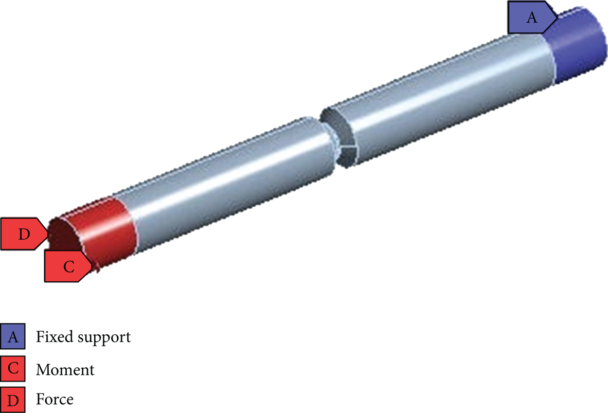
Structural analysis model of specimen.

2.1. Mesh Sensitivity Analysis

Mesh sensitivity analysis has been performed to obtain the optimum mesh size which will give a good balance between accuracy, processor time, and storage load [19]. Table 2 shows the result of the mesh sensitivity analysis. As the specimens are of similar notch size and shape, the resulting optimum mesh size is also of the same size; mesh sensitivity is not needed for individual specimens. From Table 2, it can be seen that after a mesh size of 0.175 mm the stress values do not change by an appreciable amount, but there is an exponential rise in the number of nodes and elements, which will result in an increase of the processor time and storage requirement without much increase in the accuracy of the stress results. Hence, to get the optimum performance a mesh size of 0.175 mm is selected for meshing both specimen models.

Table 2:

Mesh sensitivity analysis results.

Mesh size (mm)	von mises stress (MPa)	Tresca stress (MPa)	Max principal (MPa)	Number of nodes	Number of elements

0.1	562.96	575.72	576.27	587762	409838
0.125	562	573.85	574.53	414193	287994
0.15	561.1	572.8	574	260754	181331
0.175	560.78	572.65	575.42	176749	122197
0.2	554.79	565.7	569.95	144013	99252

3. Endurance Function Model

Brighenti and Carpinteri [8] proposed an endurance function model on the basis of a continuum damage mechanics approach, with the assumption that the whole fatigue life is crack nucleation dominated and that the fatigue life for crack propagation is negligible with respect to total life. For isotropic materials the endurance function can be expressed as below:

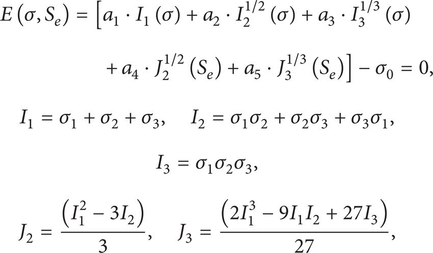
\begin{matrix} E (σ, S_{e}) = [a_{1} \cdot I_{1} (σ) + a_{2} \cdot I_{2}^{1 / 2} (σ) + a_{3} \cdot I_{3}^{1 / 3} (σ) + a_{4} \cdot J_{2}^{1 / 2} (S_{e}) + a_{5} \cdot J_{3}^{1 / 3} (S_{e})] - σ_{0} = 0, \\ I_{1} = σ_{1} + σ_{2} + σ_{3}, I_{2} = σ_{1} σ_{2} + σ_{2} σ_{3} + σ_{3} σ_{1}, \\ I_{3} = σ_{1} σ_{2} σ_{3}, \\ J_{2} = \frac{(I_{1}^{2} - 3 I_{2})}{3}, J_{3} = \frac{(2 I_{1}^{3} - 9 I_{1} I_{2} + 27 I_{3})}{27}, \end{matrix}

(1)

where a₁ to a₅ and σ₀ are the material constants, I₁, I₂, and I₃ are stress tensor invariants, and J₂, J₃ deviatoric stress invariants are functions of stress tensor σ and effective deviatoric stress tensor S_e, respectively. Here, S_e = S – S_b; that is, S is the current applied deviatoric stress tensor and S_b is the back stress tensor which measures the endurance function evolution in the stress space.

Damage is assumed to occur when E(σ, S_e) > 0 and no damage occurs when E(σ, S_e) ≤ 0, and an increment in damage will happen when dE (increment in endurance function) > 0. To define dE properly, it is specified that if there is a case where the stress value at point i results in E(σ_i, S_{e, i}) > 0 and the previous point results in E(σ_{i – 1}, S_{e, i – 1}) < 0, the quantity E(σ_{i – 1}, S_{e, i – 1}) is set equal to zero, which in turn results in keeping dE always greater than zero.

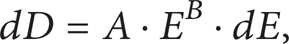
The damage D is evaluated by considering the progressive accumulation of damage increments; that is, at each load step the damage increment is equal to or greater than zero dD ≥ 0 and consequently the material damage D is a non-decreasing positive function; that is, D ≥ 0 [3]. And final collapse occurs when D reaches unity (D = 1). The damage rate dD is assumed to depend on the current value of E as well as dE, with the relationship between dD and dE as follows:

d D = A \cdot E^{B} \cdot d E,

(2)

where A and B are material constants. The stress gradient effect is taken into account by inserting a reducing factor G into (2):

d D = [A \cdot E^{B} \cdot d E] \cdot G .

(3)

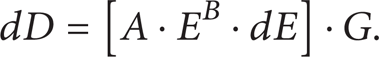
Here,

G = e^{- V \cdot γ},

(4)

where G is the notch gradient correction factor which depends on V (material constant) and the stress field parameter γ, which represents the stress gradient absolute value at the notch root. The evolution of deviatoric back stress S_b is assumed to follow the relationship below:

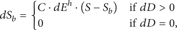
d S_{b} = {\begin{cases} C \cdot d E^{h} \cdot (S - S_{b}) & if d D > 0 \\ 0 & if d D = 0, \end{cases}

(5)

where C and h are material parameters.

3.1. Application of Genetic Algorithm for Parameter Estimation

A genetic algorithm (GA) is used to find the optimum values of these parameters. Such algorithms (random stochastic methods of global optimization) are used to minimize or maximize an objective function chosen for a given problem to be solved. Such an approach can be useful to evaluate the model parameters (in the context of model parameter tuning), once the response of the physical system to a given input is known [20]. GAs have some advantages with respect to classical techniques, as they allow us to handle problems with multiple minima and nonconvexity properties, thus avoiding numerical instability and missing the global optimum [21]. A GA can handle any kind of objective function and creates a population of solutions and applies genetic operators, such as selection, mutation, crossover, and elitism to evolve the solutions in order to find the best ones [22], by iteratively repeating the “evolution procedure” until a given tolerance is attained [23]. In order to apply the endurance function model, values of 11 parameters that need to be evaluated, as defined in (1)–(5). If the fatigue life N_f is known for the generic multiaxial stress history where damage D reaches unity, a prediction error can be defined as follows:

e = D (a_{1}, a_{2}, \dots, N_{f}) - 1,

(6)

where D(a₁, a₂, …, N_f) is the damage evaluated at N_f. The values of the model parameters can be found by minimizing this error function using the GA procedure [8].

4. Simplified Endurance Function Model

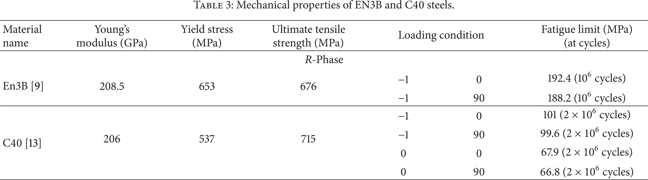
The two materials, EN3B and C40 steels, are used in this study with six sets of fatigue life data (Table 1), under cyclic multiaxial in-phase and out of phase loadings. Specimens are notched specimens as shown in Figure 1. The mechanical characteristics of both steels are as follows in Table 3 [8, 9]. Initially linear stress analysis of specimens was conducted at every set of applied stress mentioned in Table 1, and all three principal stresses (σ₁, σ₂, σ₃) were recorded at the notch root where the highest value of maximum principal stress is occurring [24, 25]. Neuber elastic plastic correction is applied where stresses are found to be above yield strength [2, 14, 26]. Stress invariants (I₁, I₂, I₃, J₂, and J₃) are then calculated from the following relationships depending on principal stresses after Neuber correction is applied where necessary [27].

Table 3:

Mechanical properties of EN3B and C40 steels.

Material name	Young's modulus (GPa)	Yield stress (MPa)	Ultimate tensile strength (MPa)	Loading condition		Fatigue limit (MPa) (at cycles)

R-Phase
En3B [9]	208.5	653	676	−1	0	192.4 (10⁶ cycles)
En3B [9]	208.5	653	676	−1	90	188.2 (10⁶ cycles)

C40 [13]	206	537	715	−1	0	101 (2 × 10⁶ cycles)
				−1	90	99.6 (2 × 10⁶ cycles)
				0	0	67.9 (2 × 10⁶ cycles)
				0	90	66.8 (2 × 10⁶ cycles)

The endurance function parameters, where G is the notch gradient correction factor, becomes G = 1 due to the fact that FEA gives the value of stress at the notch root directly. This in return nullifies the requirement to determine parameter V and the stress field parameter γ, thus reducing the number of endurance function parameters by one. For both of the considered materials EN3B and C40 steel, the cyclic behavior is assumed to be following a stable hysteresis loop, which in return allows the change in back stress dS_b = 0. Thus, there is no need to calculate parameters C and h in (5). So finally, from 11 parameters of the endurance function, the number required is reduced to eight, a₁, a₂, a₃, a₄, a₅, σ₀, A, and B.

Now, to calculate the value of parameters at calibration points (from all loading conditions considered in this study as per Table 1, the selected ones to calibrate the parameters of endurance function are called calibration points. Table 4 shows the calibration points with calibrated parameter values), GA is used where the error function which is to be minimized is defined as (7), with the assumption that, as the cyclic behavior of the material is stable, the damage in each cycle is the inverse of the fatigue life in the cycles:

e = D - \frac{1}{N_{f}},

(7)

where the damage per cycle is calculated from the endurance function. These equations are inserted in the GA algorithm for optimization of the endurance function parameters [28 –30]. Figure 3 shows the flow chart of fatigue life estimation process.

Table 4:

Parameters at of calibration points for endurance function model obtained from GA for EN3B and C40.

Load (MPa)		a ₁	a ₂	a ₃	a ₄	a ₅	σ₀	A	B
σ	τ	a ₁	a ₂	a ₃	a ₄	a ₅	σ₀	A	B

EN3B (R = – 1 and phase = 0°)
275	158.8	0.5107	1.004	0.2313	1.129	1.197	180	5.348 × 10⁻⁹	0.2299
180	103.9	0.4001	0.5233	0.4113	0.7745	0.8194	166.5	1.009 × 10⁻⁹	0.08192

EN3B (R = – 1 and phase = 90°)
285	164.5	0.4255	1.19	0.3625	1.076	0.7991	141.4	7.056 × 10⁻⁹	0.2389
200	115.5	0.2708	0.327	0.2189	0.7392	0.4868	149.7	2.882 × 10⁻⁹	0.07962

C40 (R = – 1 and phase = 0°)
200	200	0.1412	0.3676	0.4504	1.404	−0.3757	80.18	8.034 × 10⁻⁹	0.4285
101	101	0.4972	0.7769	0.3194	1.44	0.9721	85.33	1.485 × 10⁻¹⁰	0.2322

C40 (R = – 1 and phase = 90°)
199.7	199.7	0.4358	0.5965	0.6721	1.428	1.165	76.7	2.868 × 10⁻⁸	0.2134
99.6	99.6	0.2615	0.2907	0.4818	1.345	−0.2697	79.02	1.032 × 10⁻⁹	0.1377

C40 (R = 0 and phase = 0°)
158.1	158.1	0.7446	0.2931	0.432	1.731	0.2959	58.4	8.05 × 10⁻⁹	0.224
67.9	67.9	0.05374	0.5927	0.6035	0.9929	0.3145	61.08	1.609 × 10⁻⁹	0.03816

C40 (R = 0 and phase = 90°)
158	158	0.4721	0.4814	0.5829	1.655	0.7878	54.44	7.373 × 10⁻⁹	0.2677
66.8	66.8	0.1452	0.6464	0.572	0.9294	0.6613	61.83	1.198 × 10⁻⁹	0.1313

Figure 3:

Flow chart of fatigue estimation process.

The initial values table required for the GA is generated randomly from the ranges of parameters assumed. The range for σ₀ is defined with its upper limit as the conventional fatigue limit [8, 9] and the lower limit is set to be 25% less than the upper limit initially and then modified with ranges of other parameters until the combinations become stable, which results in minimum error. From being stable, it is assumed that the sets of parameter values resulting in minimum error have no significant change in respective parameters. Then, the top three values of parameters predicted for each calibration point are selected with respect to the minimum error which are weighted average on the basis of error [31], and the resulting values of weighted average are characterized as the parameters of the endurance function at the respective calibration point. Table 4 shows the parameters at the calibration points determined using the GA.

5. Results and Discussion

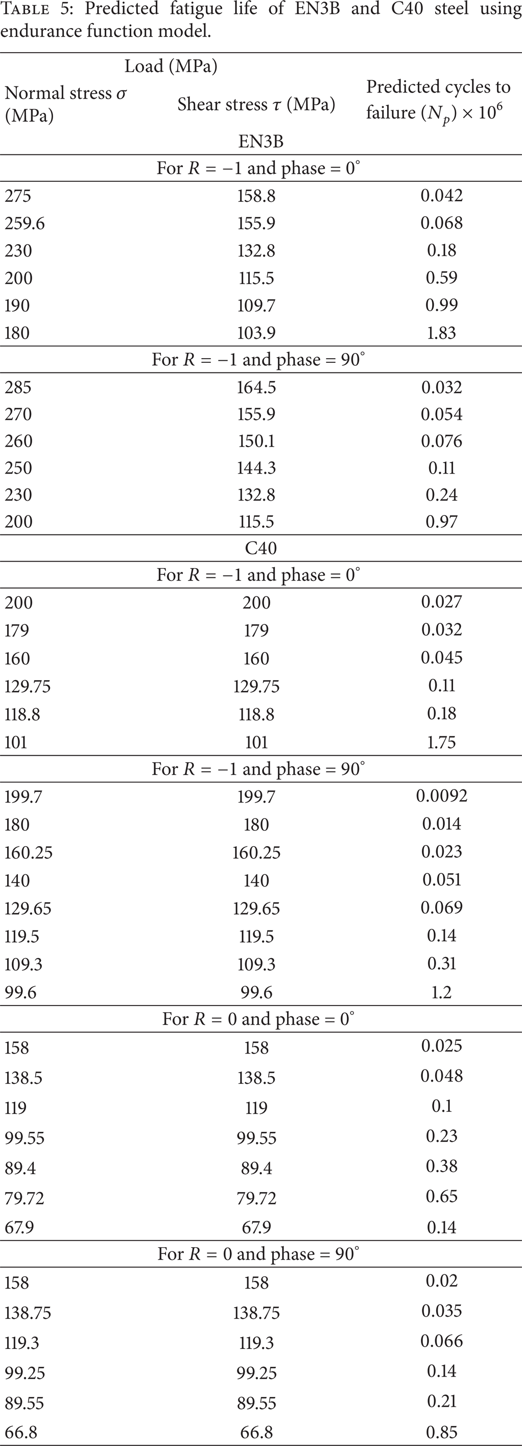
The parameters for all the calibration points calculated using the GA, as shown in Table 4 for both materials and their respective load sets, are used to determine values for other loading conditions in Table 1 by interpolation between the parameter values at calibration points; fatigue life is then estimated using the endurance function model. The predicted fatigue life is reported in Table 5. The first thing to notice from the fatigue life prediction results is that the fatigue life values calculated at the calibration points themselves are not the same as the experimental life (Tables 1, 4, and 5), which should theoretically be the same, as these points are used to calculate the coefficients for the endurance function model. The reason lies in the fact that the parameters calculated at each calibration point are the weighted average of top three values predicted by GA, which in turn allowed the estimation of fatigue life at the calibration point to deviate from the experimental life at that point. But the author suggests that this weighted average should nevertheless be used rather than just relying on one set with minimum error, so as to better capture the trend of the coefficients from the three sets from which the weighted average is being taken. The interpolation of the coefficients of the endurance function for load conditions other than calibration points is introduced, where parameter values are interpolated between the two calibration points parameter values with respect to applied load and calibration point load values, which is a better approximation for estimating the fatigue life than the proposed method of calculating only one set of coefficients [8]. Also, the idea of using the weighted average of the coefficients calculated from different load values in turn creates a bias on the basis of error towards the coefficients with minimum error, which should not be there, as all the calibration load points are experimental values and have equal weight.

Table 5:

Predicted fatigue life of EN3B and C40 steel using endurance function model.

Load (MPa)		Predicted cycles to failure (N_p) × 10⁶
Normal stress σ (MPa)	Shear stress τ (MPa)	Predicted cycles to failure (N_p) × 10⁶
EN3B

For R = – 1 and phase = 0°

275	158.8	0.042
259.6	155.9	0.068
230	132.8	0.18
200	115.5	0.59
190	109.7	0.99
180	103.9	1.83

For R = – 1 and phase = 90°

285	164.5	0.032
270	155.9	0.054
260	150.1	0.076
250	144.3	0.11
230	132.8	0.24
200	115.5	0.97

C40

For R = – 1 and phase = 0°

200	200	0.027
179	179	0.032
160	160	0.045
129.75	129.75	0.11
118.8	118.8	0.18
101	101	1.75

For R = – 1 and phase = 90°

199.7	199.7	0.0092
180	180	0.014
160.25	160.25	0.023
140	140	0.051
129.65	129.65	0.069
119.5	119.5	0.14
109.3	109.3	0.31
99.6	99.6	1.2

For R = 0 and phase = 0°

158	158	0.025
138.5	138.5	0.048
119	119	0.1
99.55	99.55	0.23
89.4	89.4	0.38
79.72	79.72	0.65
67.9	67.9	0.14

For R = 0 and phase = 90°

158	158	0.02
138.75	138.75	0.035
119.3	119.3	0.066
99.25	99.25	0.14
89.55	89.55	0.21
66.8	66.8	0.85

This also proves the applicability of interpolation between the coefficients, as this keeps the weight of the coefficients at calibration load points the same, with estimates at other points following the trend of changing the coefficients with the load values as shown in Figure 4. The stress life curves from the predicted and experimental life data for EN3B are shown in Figure 6 and for C40 steel in Figure 7. From the results, it can be seen that the endurance function with the proposed application methodology shows good agreement with experimental data for both materials in the case of in-phase loading. Brighenti et al. [32] also reported that for different materials the endurance function model behaves close to the experimental results, with loading conditions having R = – 1, which conforms with the results reported in this paper in similar loading conditions. In the out of phase case for both materials, the results are in good agreement in the low cycle region but become more conservative as we move towards the high cycle region. One reason for this is that a greater number of experimental data points are in the low cycle region, which causes the calibration of the model to be biased towards the low cycle region. Also, there is scatter in the experimental data [9, 13], as is visible in Figures 5(b) and 6(b), which can lead to error in the prediction of fatigue life.

Figure 4:

Trend of coefficients for calibration points for EN3B R = – 1 phase = 0°.

Figure 5:

S-N curve and experimental versus predicted life for EN3B steel.

Figure 6:

S-N curve and experimental versus predicted life for C40 steel.

Figure 7:

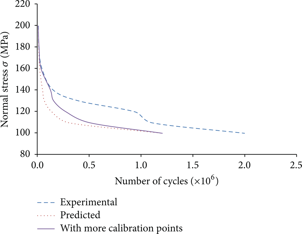
S-N curves for C40 steel for R = – 1 and phase 90° with predicted curve from one more calibration point.

One simple solution to improve the prediction accuracy is to increase the number of calibration points, which will lead to better capture of the change in the experimental S-N curve trend, as shown in Figure 7. Here, one more calibration point is included with loading condition normal stress σ_a and shear stress τ_a = 140 MPa with R = – 1 and phase = 90° for C40 specimen (Table 1), which clearly resulted in improved agreement with the experimental S-N curve. So, it can be deduced from this that the data set required for the endurance model to work properly should have more data points and in both the low and high cycle regions, so that more calibration points can be used to fit the endurance model with the experimental data. The data set used in this study is small in size, which is why only one extra calibration point is included to check this hypothesis, and the results show that the idea of more calibration points will indeed work well. So, from these results, we can conclude that the methodology defined in this study can lead us to a model which works well in both the low and high cycle regions.

6. Conclusion

A methodology has been proposed to apply the endurance function model with a GA to estimate fatigue life. The proposed methodology included application of FEA, which in turn simplified the endurance function model by reducing one coefficient for the notch gradient correction factor. Also, application of FEA resulted in a simplified method for determining the stress tensor and deviatoric stress invariants. An interpolation technique is introduced in the proposed methodology to estimate the coefficients at each load point using calibration point coefficients, which resulted in better representation of the fatigue behavior from the endurance function model. The results show that the endurance function model is in good agreement with experimental fatigue life data for in-phase loading and also to some extent for out of phase loading, but, due to having fewer data points in the experimental data, the high cycle region is not accurately predicted. The scheme to use more than two calibration points for one data set shows improved prediction of the fatigue life. From the study, it is concluded that the proposed methodology for the endurance function model resulted in accurate prediction of fatigue life for the stable fatigue life behavior of the material. However, further development is needed to accommodate the nonlinear behavior of the material in order to extend the application region of the endurance function model with the proposed methodology to include variable amplitude and random loading cases.

Footnotes

Nomenclature

References

Lee

Pan

Hathaway

, and Barkey

, Fatigue Testing and Analysis: Theory and Practice, Butterworth Heinemann, New York, NY, USA, 2005.

Stephens

R. I.

Fatemi

Stephens

R. R.

, and Fuchs

H. O.

, Metal Fatigue in Engineering, John Wiley & Sons, New York, NY, USA, 2000.

Manson

S. S.

and Halford

G. R.

, Fatigue and Durability of Structural Materials, ASM International, Materials Park, Ohio, USA, 2006.

Rahman

M. M.

Ariffin

A. K.

Jamaludin

, and Haron

C. H. C.

, “Influence of surface treatments on fatigue life of a two-stroke free piston linear engine component using random loading,” Journal of Zhejiang University Science A, vol. 7, no. 11, pp. 1819–1830, 2006.

Rahman

M. M.

Ariffin

A. K.

Jamaludin

, and Haron

C. H. C.

, “Finite element based durability assessment of a free piston linear engine component,” Structural Durability and Health Monitoring, vol. 3, no. 1, pp. 1–13, 2007.

Rahman

M. M.

Kadirgama

Noor

M. M.

Rejab

M. R. M.

, and Kesulai

S. A.

, “Fatigue life prediction of lower suspension arm using strain-life approach,” European Journal of Scientific Research, vol. 30, no. 3, pp. 437–450, 2009.

Rahman

M. M.

Ariffin

A. K.

Rejab

M. R. M.

Kadirgama

, and Noor

M. M.

, “Multiaxial fatigue behavior of cylinder head for a free piston linear engine,” Journal of Applied Sciences, vol. 9, no. 15, pp. 2725–2734, 2009.

Brighenti

and Carpinteri

, “A notch multiaxial-fatigue approach based on damage mechanics,” International Journal of Fatigue, vol. 39, pp. 122–133, 2012.

Susmel

and Taylor

, “The modified Wohler curve method applied along with the theory of critical distances to estimate finite life of notched components subjected to complex multiaxial loading paths,” Fatigue & Fracture of Engineering Materials & Structures, vol. 31, no. 12, pp. 1047–1064, 2008.

10.

Macha

and Nieslony

, “Critical plane fatigue life models ofmaterials and structures under multiaxial stationary random loading: the state-of-the-art in Opole Research Centre CESTI and directions of future activities,” International Journal of Fatigue, vol. 39, pp. 95–102, 2012.

11.

Susmel

and Tovo

, “Estimating fatigue damage under variable amplitude multiaxial fatigue loading,” Fatigue & Fracture of Engineering Materials & Structures, vol. 34, no. 12, pp. 1053–1077, 2011.

12.

Susmel

and Taylor

, “A critical distance/plane method to estimate finite life of notched components under variable amplitude uniaxial/multiaxial fatigue loading,” International Journal of Fatigue, vol. 38, pp. 7–24, 2012.

13.

Atzori

Berto

Lazzarin

, and Quaresimin

, “Multiaxial fatigue behaviour of a severely notched carbon steel,” International Journal of Fatigue, vol. 28, no. 5–6, pp. 485–493, 2006.

14.

Bishop

N. W. M.

and Sherratt

, Finite Element Based Fatigue Calculations, NAFEMS, 2000.

15.

Rahman

M. M.

Ariffin

A. K.

Abdullah

Noor

M. M.

, and Rosli

A. B.

, “Durability assessment of cylinder block for two stroke free piston linear engine using random loading,” American Journal of Applied Sciences, vol. 6, no. 4, pp. 726–735, 2009.

16.

Rahman

M. M.

Ariffin

A. K.

Jamaludin

Abdullah

, and Noor

M. M.

, “Finite element based fatigue life prediction of a new free piston engine mounting,” Journal of Applied Sciences, vol. 8, no. 9, pp. 1612–1621, 2008.

17.

Rahman

M. M.

Ariffin

A. K.

Abdullah

Noor

M. M.

Bakar

R. A.

, and Maleque

M. A.

, “Finite element based fatigue life prediction of cylinder head for two-stroke linear engine using stress-life approach,” Journal of Applied Sciences, vol. 8, no. 19, pp. 3316–3327, 2008.

18.

Ottosen

N. S.

Stenstrom

, and Ristinmaa

, “Continuum approach to high-cycle fatigue modeling,” International Journal of Fatigue, vol. 30, no. 6, pp. 996–1006, 2008.

19.

Kamal

Rahman

M. M.

, and Rahman

A. G. A.

, “Fatigue life evaluation of suspension knuckle using multi body simulation technique,” Journal of Mechanical Engineering and Sciences, vol. 3, no. 1, pp. 291–300, 2012.

20.

Brighenti

Carpinteri

, and Vantadori

, “A genetic algorithm applied to optimisation of patch repairs for cracked plates,” Computer Methods in Applied Mechanics and Engineering, vol. 196, no. 1–3, pp. 466–475, 2006.

21.

Davis

, Ed., Handbook of Genetic Algorithms, Van Nostrand Reinhold, New York, NY, USA, 1991.

22.

Franulovic

Basan

, and Prebil

, “Genetic algorithm in material model parameters' identification for low-cycle fatigue,” Computational Materials Science, vol. 45, no. 2, pp. 505–510, 2009.

23.

Gantovnik

V. B.

Anderson-Cook

C. M.

Gürdal

, and Watson

L. T.

, “A genetic algorithm with memory for mixed discrete-continuous design optimization,” Computers and Structures, vol. 81, no. 20, pp. 2003–2009, 2003.

24.

Rahman

M. M.

Ariffin

A. K.

Rejab

M. R. M.

Kadirgama

, and Noor

M. M.

, “Multiaxial fatigue behavior of cylinder head for a free piston linear engine,” Journal of Applied Sciences, vol. 9, no. 15, pp. 2725–2734, 2009.

25.

Rahman

M. M.

Kadirgama

Noor

M. M.

Rejab

M. R. M.

, and Kesulai

S. A.

, “Fatigue life prediction of lower suspension arm using strain-life approach,” European Journal of Scientific Research, vol. 30, no. 3, pp. 437–450, 2009.

26.

Society of Automotive Engineers (SAE), “Low cycle fatigue properties ferrous and non-ferrous materials,” Tech. Rep. SAE J1099, Society of Automotive Engineers, 2002.

27.

Socie

D. F.

and Marquis

G. B.

, Multiaxial Fatigue, Society of Automotive Engineers, Warrendale, Pa, USA, 2000.

28.

Clarich

Russo

, and Carriglio

, “Multi-objective optimization with modeFRONTIER interfaces for ANSA and μETA Post,” in Proceedings of the 4th ANSA & μETA International Conference, Thessaloniki, Greece, 2011.

29.

Perillo

Primavera

Fuligno

Fabbri

Steenbergen

, and Pasini

, “Optimization and robustness of complex material model simulations with modeFRONTIER,” in Proceedings of the 7th European LS-DYNA Conference, pp. 1–10, Salzburg, Austria, 2009.

30.

modeFRONTIER 4.1 User Manual, ESTECO, Trieste, Italy, http://www.esteco.com/modefrontier.

31.

Hariharan

Prakash

R. V.

, and Sathya Prasad

, “Weighted error criterion to evaluate strain-fatigue life prediction methods,” International Journal of Fatigue, vol. 33, no. 5, pp. 727–734, 2011.

32.

Brighenti

Carpinteri

, and Corbari

, “Damage mechanics and Paris regime in fatigue life assessment of metals,” International Journal of Pressure Vessels and Piping, vol. 104, pp. 57–68, 2013.

Fatigue Life Prediction Using Simplified Endurance Function Model

Abstract

1. Introduction

2. Finite Element Modeling and Analysis

2.1. Mesh Sensitivity Analysis

3. Endurance Function Model

3.1. Application of Genetic Algorithm for Parameter Estimation

4. Simplified Endurance Function Model

5. Results and Discussion

6. Conclusion

Footnotes

Nomenclature

References