Sage Journals: Discover world-class research

Abstract

This is a mathematic model for the optimal operation of the gathering pipeline network and its solution provides this gathering pipeline network having a triple-line heat-tracing process, a method for reducing the operational costs and increasing economic benefit. The model consists of an objective function, minimum total operation cost, and 3 constraints including water temperature constraint at pipe nodes, inlet oil temperature constraints, and outlet water temperature constraint. By using a sequential quadratic programming algorithm, the model can be solved and a set of optimal mass rate and the desired temperature of tracing water are attained. The method is here specifically applied to the optimal operation analysis of a gathering pipeline network in North China Oilfield. The result shows its operation cost can be reduced by 2076RMB/d, which demonstrates that this method contributes to the production cost reduction of old oilfields in their high water-cut stage.

1. Introduction

Triple-line process has been widely used in early oilfield development in China. With oilfields now entering the high water-cut stage, it has become more and more clear that the triple-line process has the disadvantages of high energy consumption and low efficiency. In the last twenty years, research has been mostly based on the optimal design of pipeline network [1 –4] and the simulation of pipeline network [5 –7], but seldom on optimal operation problems of triple-line process. On the condition that the triple-line process is not changed, research was carried out on optimizing the operation parameters of oilfield gathering and transportation system which had positive effects on cost reduction and economic benefit increases for those areas unsuited to the low-temperature gathering and transportation process.

2. Thermodynamic Calculation of Tracing Oil Pipelines

The cross-section of the tracing oil pipelines is divided into 5 parts [8] (Figure 1). S¹ is the heat transfer surface between an oil pipeline and the soil, S² is the heating surface between the pipes' interspace and the soil, S³ is the heat transfer surface between a water pipeline and the soil, S⁴ is the heat transfer surface between an oil pipeline and the pipes' interspace, andS⁵ is the heat transfer surface between a water pipeline and the pipes' interspace. By solving the pipe element thermodynamic differential equation [9], Oil/water temperature at the end of the oil/water pipeline can be obtained asshown in Figure 1, where S¹ … S⁵ are the areas of 5 heat transfer surfaces of unit pipe length, m² Consider.

T^{Z} = D^{1} e^{r^{1} L} + D^{2} e^{r^{2} L} + t^{f},

(1)

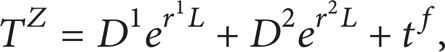
whereT^z is the liquid temperature at the end of the oil pipe, °C. t^f is the average soil temperature at the depth of pipes,°C

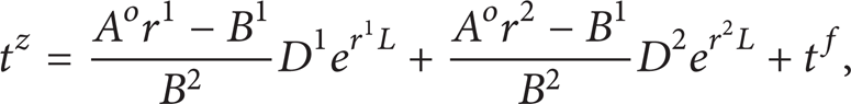
t^{z} = \frac{A^{o} r^{1} - B^{1}}{B^{2}} D^{1} e^{r^{1} L} + \frac{A^{o} r^{2} - B^{1}}{B^{2}} D^{2} e^{r^{2} L} + t^{f},

(2)

where t^z is the water temperature at the end of a tracing pipe, °C.

Figure 1:

Cross-section diagram for tracing oil pipelines.

r¹, r²,D¹, andD² are given by

r^{1,2} = \frac{- p \pm \sqrt{p^{2} - 4 q}}{2}, \begin{matrix} D^{1} = \frac{1}{A^{o} (r^{1} - r^{2})} \times [(B^{1} - A^{o} r {}^{2}) T^{q} + B^{2} t^{q} + (B^{3} + A^{o} r^{2}) t^{f}], \end{matrix}

(3)

where T^q is the liquid temperature at the beginning of an oil pipe, °C. t^q is the water temperature at the beginning of a tracing pipe, °C,

D^{2}  =  \frac{1}{A^{o} (r^{1} - r^{2})} [(A^{o} r^{1} - B^{1}) T^{q}  -  B^{2} t^{q}  -  (B^{3}  +  A^{o} r^{1}) t^{f} ],

(4)

p = \frac{C^{1}}{A^{w}} - \frac{B^{1}}{A^{o}},

(5)

q = \frac{C^{2} B^{2} - C^{1} B^{1}}{A^{w} A^{o}},

(6)

A^{o} = G c^{o},

(7)

where c^o is the specific heat of an oil pipe liquid, J/(°C · kg) Consider

A^{w} = g^{w} c^{w},

(8)

where c^w is the specific heat of water, J/(°C · kg). g^w is the mass rate of water, kg/s Consider

B^{1} = \frac{{(K^{4} S^{4})}^{2}}{K^{2} S^{2} + K^{4} S^{4} + K^{5} S^{5}} - K^{1} S^{1} - K^{4} S^{4},

(9)

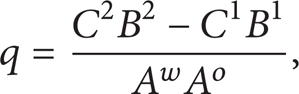
where K¹ … K⁵ are the overall heat transfer coefficients of 5 heat transfer surfaces, W/(m² ·°C),

\begin{matrix} B^{2} = \frac{K^{4} S^{4} \cdot K^{5} S^{5}}{K^{2} S^{2} + K^{4} S^{4} + K^{5} S^{5}}, \\ B^{3} = K^{1} S^{1} + \frac{K^{4} S^{4} \cdot K^{2} S^{2}}{K^{2} S^{2} + K^{4} S^{4} + K^{5} S^{5}}, \\ C^{1} = \frac{- {(K^{5} S^{5})}^{2}}{K^{2} S^{2} + K^{4} S^{4} + K^{5} S^{5}} + K^{3} S^{3} + K^{5} S^{5}, \\ C^{2} = - \frac{K^{4} S^{4} \cdot K^{5} S^{5}}{K^{2} S^{2} + K^{4} S^{4} + K^{5} S^{5}}, \\ C^{3} = - (K^{3} S^{3} + \frac{K^{2} S^{2} \cdot K^{5} S^{5}}{K^{2} S^{2} + K^{4} S^{4} + K^{5} S^{5}}) . \end{matrix}

(10)

3. Thermodynamic Calculation of Pipeline Network

3.1. Pipe Network Numbering Method

The oil wells, the metering stations, the transfer station, and the pipelines connecting them are ranked and numbered with the following rules. The transfer station is level 0 node, with no subscript; the metering station is level 1 node, with subscript i as its number; the oil well is level 2 node, with subscript ij as its number. A transfer station is the highest level, a metering station comes second, and an oil well is the lowest. The number of pipelines connecting two nodes follows the lower one. n is the total number of metering stations, and m_i is the total number of oil wells connected with the metering station i. As shown in Figure 2, the transfer station has 2 metering stations, one of them has 3 wells and the other has 2.

Figure 2:

Pipe network numbering method.

3.2. Node Parameters Calculation of Heat Tracing Pipelines

(1) Mass rate and specific heat of an oil pipe liquid at nodes:

\begin{matrix} G_{i j} = Q_{i j} \cdot w_{i j} \cdot ρ^{w} + Q_{i j} \cdot (1 - w_{i j}) \cdot ρ^{o}, \\ G_{i} = \sum_{j = 1}^{m_{i}} G_{i j}, \end{matrix}

(11)

where G_i/G_ij is the mass rate of an oil pipe's liquid i/ij, kg/s. ρ^w is the water density, kg/m³. ρ^o is the crude density, kg/m³.Q_ij is the volumetric flow rate of an oil pipe liquid ij, m³/s. w_ij is the volumetric water cut of a well ij,

\begin{matrix} c_{i j}^{o} = \frac{Q_{i j} \cdot w_{i j} \cdot ρ^{w} \cdot c^{w} + Q_{i j} \cdot (1 - w_{i j}) \cdot ρ^{o} \cdot c^{o}}{Q_{i j} \cdot w_{i j} \cdot ρ^{w} + Q_{i j} \cdot (1 - w_{i j}) \cdot ρ^{o}}, \\ c_{i}^{o} = \frac{\sum_{j = 1}^{m_{i}} c_{i j}^{o} G_{i j}}{G_{i}}, \end{matrix}

(12)

where c_i^o/c_ij^o is the specific heat of an oil pipe's liquid i/ij, J/(°C · kg).

(2) Temperature of an oil pipe liquid at nodes:

T_{i}^{q} = \frac{\sum_{j = 1}^{m_{i}} c_{i j}^{o} G_{i j} T_{i j}^{z}}{c_{i}^{o} G_{i}}

(13)

T_i^q is the resulting oil pipes' liquid temperature when mixed at their node i, °C. T_ij^z is the liquid temperature at the end of an oil pipe ij, °C.

(3) Temperature of a water pipe liquid at nodes

t_{i}^{q} = \frac{\sum_{j = 1}^{m_{i}} g_{i j}^{w} t_{i j}^{z}}{g_{i}^{w}},

(14)

where t_ij^z is the water temperature at the end of a tracing pipe ij, °C. t_i^q is the resulting tracing pipes' water temperature when mixed at their node i, °C. g_i^w/g_ij^w is the mass rate of water distributed to a node i/ij, kg/s.

3.3. Node Parameters Calculation of Water Pipeline Network

Mass Rate of Water at the Nodes. The mass rate of water at a node is calculated serially from the lower level to the higher one:

g_{i}^{w} = \sum_{j = 1}^{m_{i}} g_{i j}^{w}, g_{}^{w} = \sum_{i = 1}^{n} g_{i}^{w} .

(15)

Water Temperature at Nodes. Water temperature at a node is calculated by using the Sukhov Formula serially from the lower level to the higher one:

\begin{matrix} t_{i j}^{Q} = (t_{i j} - t^{f}) e^{(K_{i j} π d_{i j} / g_{i j}^{w} c^{w}) L_{i j}} + t^{f}, \\ t_{i}^{Q} = (t_{i} - t^{f}) e^{(K_{i} π d_{i} / g_{i}^{w} c^{w}) L_{i}} + t^{f}, \end{matrix}

(16)

where t_i^Q/t_ij^Q is the water temperature at the beginning of a water pipe i/ij, °C. $t_{i}^{} / t_{i j}^{}$ is the water temperature at the end of a water pipe i/ij, °C. K_i/K_ij is the overall heat transfer coefficient of a water pipe i/ij, W/(m² · °C). d_i/d_ij is the diameter of the water pipe i/ij, m. L_i/L_ij is the length of the water pipe i/ij, m.

4. Optimal Mathematic Model

4.1. Objective Function

With a water mass rate {g_ij} and a water temperature {t_ij} as decision variables and the minimum total operation cost, including heating cost and power cost, as the target, assuming that ΔH is a known quantity, the objective function is given by

\min F ({g_{i j}}, {t_{i j}}) = \frac{p^{r} c^{w} g^{w} (t - t^{y})}{q^{r} η} + \frac{p^{d} g^{w} g Δ H}{η^{'}},

(17)

where p^r is the fuel price, RMB/kg. p^d is the price of electricity RMB/J.t^y is the water temperature before heated, °C. g is the acceleration of gravity, N/kg. ΔH is the water head of the pump, m. q^r is the lower heating value, J/kg. η is the efficiency of heating furnace. η′ is the pump's efficiency.

4.2. Constraints Condition

Water Temperature Constraint at the Nodes. One node has multiple outlets. The water temperatures of these outlets are the same:

Δ t_{i}^{} = 0, Δ t_{i j}^{} = 0,

(18)

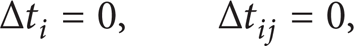
where Δt_i is the commencing temperature difference between a water pipe i and a water pipe (i + 1),°C. Δt_ij the commencing temperature difference between a water pipe ij and a water pipe i(j + 1),°C.

Inlet Oil Temperature Constraint. To ensure the safe operation of the pipeline, the minimum inlet temperature [10] is specified to be higher than the freezing point of crude oil:

T_{i}^{Z} \geq T^{n} + Δ t,

(19)

where T_i^z is the transfer station's inlet temperature of an oil pipe i, °C. Tⁿ is the freezing point of crude oil, °C.Δt is the temperature allowance, °C.

Outlet Water Temperature Constraint. The outlet water temperature of the transfer station is usually (90 ~ 100)°C [11, 12]:

t \leq 100,

(20)

where t is the outlet water temperature of a transfer station, °C.

5. Model Solutions

There are n metering stations, $\sum_{i = 1}^{n} m_{i}$ oil wells in this model, and correspondingly, $2 \times \sum_{i = 1}^{n} m_{i}$ decision variables, $\sum_{i = 1}^{n} m_{i} - 1$ equality constraints and (n + 1) inequality constraints are generated. The model is a highly nonlinear problem, of which the most common method used to solve is the sequential quadratic programming algorithm. The sequential quadratic programming algorithm is a fast and effective method, of which the convergence rate is proved to be superliner under certain conditions [13, 14].

5.1. Sequential Quadratic Programming Algorithm

The main idea of the algorithm is to build a simple series of approximate optimization problems, namely, quadratic programming problems, using the information from the original nonlinear program. By solving these new problems, current iteration can be updated and gradually approximate the solution of the original nonlinear programming problem [15]. At the kth step, the approximate programming problem is asfollow:

\min q (d) = d^{T} \nabla f (x) + \frac{1}{2} d^{T} B d s . t . d^{T} \nabla c_{i} (x) + c_{i} (x) = 0, i \in E, d^{T} \nabla c_{j} (x) + c_{j} (x) \geq 0, j \in I,

(21)

where d is the difference between former and later iterations, named iteration direction; q(d) is the objective function of new programming; f(x)/c_i(x) is the objective function/constraints of original programming; ∇ f(x)/ ∇ c_i(x) is the gradient of f(x)/c_i(x); B is Hessian matrix of f(x); E/I is the set of subscripts of equality/inequality constraints.

As shown in Figure 3, the algorithm mainly includes 3 steps: (a) solve the subproblem with active-set method to get d and Lagrange multiplier λ; (b) employ quadratic interpolation and linear search to get step length α; (c) update Hessian matrix B with BFGS (Broyden-Fletcher-Goldfarb-Shanno) method, where k is the number of iterations, s is the difference between former and later iterations, and e is the control error.

Figure 3:

Main framework of the algorithm.

5.2. Active-Set Method

Subproblem (21) is a standard quadratic programming problem. The active-set method is the key to solving such problems. By swapping in/out the inequality constraints according to some rules, A convex quadratic programming (22) only with equality constraints is obtained:

\min q (d d) = d d^{T} g^{k} + \frac{1}{2} d d^{T} B d d s . t . d d^{T} \nabla c_{i} {(x)}^{k} = 0, i \in E, d d^{T} \nabla c_{j} {(x)}^{k} = 0, j \in I^{*},

(22)

where

g^{k} = B d + \nabla f (x) .

(23)

Problem (22) converts the solution of d into the solution of the direction of d, named dd.

Figure 4 gives the steps of the solution of d.

Figure 4:

Program chart of active set algorithm.

6. Example Analyses

As shown in Figure 5, the transfer station of North China Oilfield has 3 metering stations and 18 oil wells. The well effluent of each well has a mass rate of 10.5~53.6 t/d, a water cut of higher than 80%, and a temperature of 30~40°C.

Figure 5:

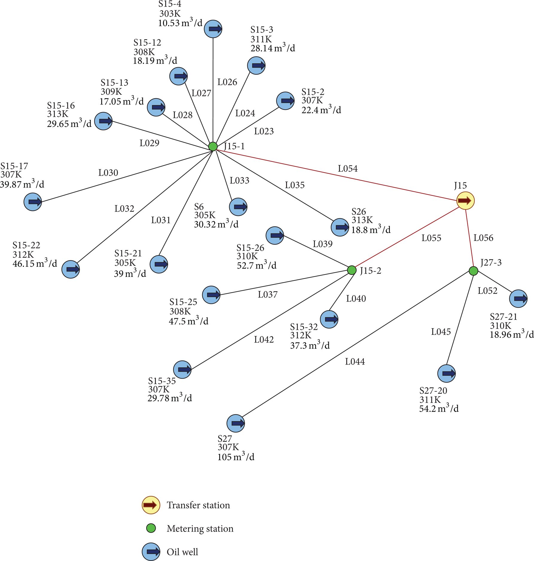
Gathering and transferring pipe network's structure.

The model has 36 decision variables, 17 equality constraints, and 4 inequality constraints. It takes 114 iterations, about 4.24 seconds to get the optimal results, as shown in Table 1.

Table 1:

Optimal operational parameters.

Well	Water mass rate (t/d)		Water temperature (°C)
Well		Before	After	Before	After

s15-2	115.5	77.0	75	79
s15-3	94.7	79.0	75	79
s15-4	44.2	34.0	70	73
s15-12	55.4	39.5	74	78
s15-13	50.2	45.7	75	79
s15–16	74.4	56.0	75	79
s15–17	111.3	79.5	75	79
s15–21	224.7	149.8	75	79
s15–22	166.3	151.3	76	80
s6	120.2	87.1	76	81
s26	76.6	46.3	73	77
s15–25	129.9	77.8	75	79
s15–26	194.5	104.5	75	79
s15–32	83.7	67.0	75	79
s15–35	127.0	86.4	74	77
s27	241.9	216	72	76
s27-20	186.7	121.2	74	78
s27-21	62.8	48.0	74	77

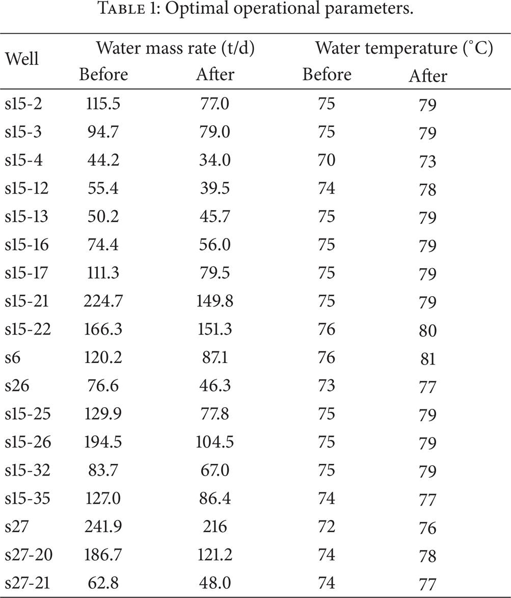
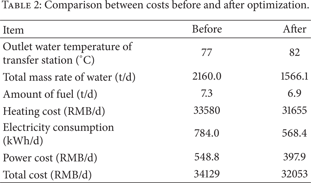
Table 2 sets out the comparison between costs before and after optimization. It shows that the optimized heating cost and power cost decrease by 1925 RMB/d and 151 RMB/d, respectively, which means the total cost can be reduced by 2076 RMB/d in sum.

Table 2:

Comparison between costs before and after optimization.

Item	Before	After

Outlet water temperature of transfer station (°C)	77	82
Total mass rate of water (t/d)	2160.0	1566.1
Amount of fuel (t/d)	7.3	6.9
Heating cost (RMB/d)	33580	31655
Electricity consumption (kWh/d)	784.0	568.4
Power cost (RMB/d)	548.8	397.9
Total cost (RMB/d)	34129	32053

7. Conclusions

A mathematic model of the gathering pipeline network optimal operation and its solution are given in this paper, which can provide optimal operation parameters for triple-line process.

Using a gathering pipeline network of North China Oilfield as an example, a mathematic model has been established. After comparing the optimal results with the actual operation data, it concludes that by using the new model, there is a considerable cost saving in accordance with the optimized parameters over that which exists at present.

Footnotes

Nomenclature

References

Barnes

R. J.

Kokossis

, and Shang

, “An integrated mathematical programming approach for the design and optimisation of offshore fields,” Computers and Chemical Engineering, vol. 31, no. 5–6, pp. 612–629, 2007.

Antonenko

D. A.

Pavlov

V. A.

Surtaew

V. N.

, and Sevastyanova

K. K.

, “Selecting an optimal field development strategy for the vankor oilfield using an integrated-asset-modeling approach,” in Proceedings of the SPE Europec/EAGE Conference and Exhibition, Rome, Italy, June 2008.

Liu

and Chen

, “Optimal parameters design of oilfield surface pipeline systems using fuzzy models,” Information Sciences, vol. 120, no. 1, pp. 13–21, 1999.

Van Den Heever

S. A.

and Grossmann

I. E.

, “An iterative aggregation/disaggregation approach for the solution of a mixed-integer nonlinear oilfield infrastructure planning model,” Industrial and Engineering Chemistry Research, vol. 39, no. 6, pp. 1955–1971, 2000.

Duan

J. M.

Wang

Zhang

, “Calculation on inner wall temperature in oil-gas pipe flow,” Journal of Central South University of Technology, vol. 19, pp. 1932–1937, 2012.

Floquet

Joulia

Vacher

Gainville

, and Pons

, “Numerical and computational strategy for pressure-driven steady-state simulation of oilfield production,” Computers and Chemical Engineering, vol. 33, no. 3, pp. 660–669, 2009.

Alvarez

C. J.

Al-awwami

M. H.

, and Aranco

, “Wet crude transport through a complex hilly terrain pipeline network,” in Proceedings of the SPE Annual Technical Conference and Exhibition, Houston, Tex, USA, October 1999.

Wang

W. X.

, Operation optimization and project setting for heavy oil three pipe tracing gathering and transferring system [M.S. thesis], Daqing Petroleum Institute, Daqing, China, 2006.

Department of Mathematics at Tongji university, Advanced Mathematics[M], Higher Education Press, Beijing, China, 2007.

10.

Gao

X. L.

and Kuang

, “The determination on the minimum allowable inlet temperature of waxy crude oil pipeline,” Oil & Gas Storage and Transportation, vol. 21, no. 11, pp. 17–21, 2002.

11.

The Writing Committee of Technical Manual of Oilfield Oil-gas Gathering and Transportation Design, Technical Manual of Oil-field Oil-Gas Gathering and Transportation Design, Petroleum Industry Press, Beijing, China, 1994.

12.

GB 50350-2005, Code for Design of Oil-Gas Gathering and Transportation System, GB, Beijing, China, 2005.

13.

G. P.

Gao

Z. Y.

, and Zheng

Y. G.

, “An effective sequential quadratic programming algorithm for nonlinear optimization problems,” Numerical Mathematics a Journal of Chinese Universities (English Series), no. 1, pp. 34–51, 2002.

14.

, “A new inexact sequential quadratic programming algorithm,” Numerical Mathematics a Journal of Chinese Universities (English Series), no. 1, pp. 1–12, 2002.

15.