Sage Journals: Discover world-class research

Abstract

The objective of this paper is the simulation of some different types of elements for semitrailers, like the suspension, both mechanical with springs and pneumatic with a spring anddiapresses; other parts like the wheels, the torsion bars, the fifth wheel and the suspension of the tractor unit have also been simulated. Then, the numerical simplified FE model of these elements that allows simulating the real behavior of the suspension to apply adequately the boundary conditions of a heavy vehicle has been obtained for a structural simulation using numerical tools with a good accuracy of the local and global behavior of the vehicle.

1. Introduction

For a good structural design of any type of structure, it is necessary to know its behavior for all possible load cases, both extreme and usual, which it can support during its useful life, and, so, the boundary conditions for each load case must be perfectly defined to have a good accuracy of the real behavior. For the particular case of semitrailers, during the structural design, the structural behavior in terms of strength and stiffness for the entire vehicle and for its parts must be optimized to obtain a lightened vehicle that can support the loads that can appear during its useful life [1]. Nowadays, numerical tools like the finite elements method are usually involved in the structural design process, but some problems related to the simulation of the boundary conditions can appear, especially for a correct simulation of some kind of elements such as the suspensions and the fifth wheel with a low computational cost. These elements can be simulated using a numerical mesh model comprising all their elements, parts, and their joints, but then the computational cost, in terms of CPU time and hardware required, and the numerical complexity of the model increase excessively [2]. The objective of this paper is the simulation of these elements using simple elements (like beams and springs) and joints to model their real behavior with a low computational cost and a low complexity. By this way, numerical simplified models, for a mechanical suspension, for a pneumatic suspension, for the fifth wheel, and for the torsion bar, have been developed.

2. Fifth Wheel Simulation

The fifth wheel is a mechanical part, located in the rear part of the tractor unit of a trailer designed to join the tractor unit to the semitrailer, allowing some relative rotations so that the vehicle can maneuver easily and does not behave like a rigid element, which would imply high efforts for the structure.

The fifth wheel has a surface with a high stiffness, named fifth wheel plate, designed to contact the king-pin sheet, and a structure that fixes this part with the rear crossbar of the tractor unit, allowing some rotations (see Figure 1) [3].

Rotation in the “X” direction of ±5°, it allows the swaying between the cabin and the semitrailer. Then the efforts due to terrains with different inclination are smaller, and there is a better contact between the wheels and the road. The geometry of the fifth wheel limits this rotation to ±5°.

Rotation in the “Y” direction of ±15°, it allows the pitch between the cabin and the semitrailer. Then the efforts due to terrains with different inclination are smaller, and there is a better contact between the wheels and the road. The geometry of the fifth wheel limits this rotation to ±15°.

Rotation in the “Z” direction of ±360° is disabled for the possible contact between both parts of the trailer, but that cannot be taken in consideration because this contact does not appear during the structural design. The objective of this rotation is to allow a higher maneuverability of the vehicle. This is due to the joint between the fifth wheel and the king-pin located in the semitrailer.

Figure 1:

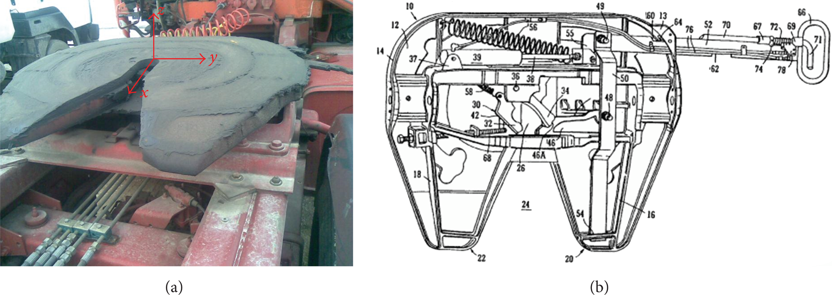
Fifth wheel coupled in a tractor cabin and their rotation directions in (a). In (b) a scheme of a fifth wheel.

The joint between the fifth wheel and the semitrailer is due to the use of the king-pin (see Figure 2) which is a piece welded to the semitrailer that allows the “Z” rotation.

Figure 2:

A fifth wheel (a), the coupling between the king-pin and the fifth wheel (b), and a king-pin (c).

Under the fifth wheel it is the crossbar of the tractor unit and its suspension that must be simulated. If we analyze the stiffness of all the parts, the stiffness of the fifth wheel and that of the crossbar are quite higher than the stiffness of the suspension [4], so they are negligible for the calculation, and only the stiffness of the suspension can be considered.

Three different fifth wheel models have been made:

model with the king-pin clamped,

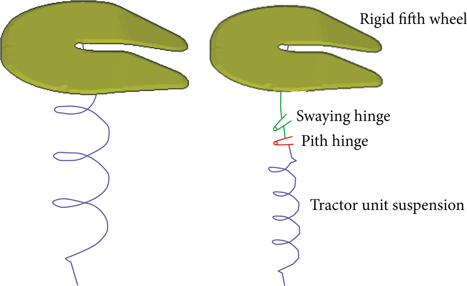
fifth wheel model with five springs (see Figure 6(right panel)),

fifth wheel model with connector (see Figure 6(left panel)).

2.1. Model with the King-Pin Clamped

This is a model that does not simulate the behavior of the fifth wheel, and it is used to compare the local and global behavior with the other models, mainly to analyze the stress concentrations near the clamps. This model does not take into consideration the behavior of the tractor unit cabin, so results obtained with it can be used to compare the global and local strength behavior far from the clamps and its deformation, but not its local behavior and the vertical displacement near the clamps.

This model is the simplest and needs low numerical requirements. Nevertheless it presents the lowest accuracy.

The main problem of this model is the local stress concentration near the fifth wheel clamp, but it can be used to analyze the rest of the vehicle because its structural behavior will be quite similar to the real one and the maximum deformation can also be obtained with it.

In this model, although all the displacements of the nodes of the king-pin are clamped, their rotations are allowed like in the real model but without the ±5° and ±15° restrictions.

Figure 3 shows the model with the king-pin clamped for a tanker.

Figure 3:

Tanker with the king-pin clamped.

2.2. Fifth Wheel Model with Five Springs

A new fifth wheel model has been made to correct the disadvantages of the previous model, but this implies that higher complexity, higher numerical requirements, and smaller increments are needed during the numerical convergence process.

In this model the fifth wheel plate was simulated like a 450 mm round rigid plate chamfered in its contour (in ABAQUS, R3D4 elements with a central reference node were used). A rigid part, like the fist model, must have a reference node, in this case located in the center, and this node must be joined to some nodes located in the center of the king-pin to constrain the relative displacements, but not the rotations (in ABAQUS a link type multipoint constraint or MPC has been used).

Then, all the rotations between the semitrailer and the tractor unit are allowed, not the displacements. To avoid the rotations without stops in “X” and in “Y” directions, a contact has been used between the king-pin sheet and the fifth wheel (in ABAQUS using a rigid to deformable contact). This contact also allows the fifth wheel to contact with the king-pin sheet only at those zones where this contact really exists, so the local stresses due to the clamp will be reduced, and the efforts will be distributed in a higher area, which is more approximated to what really occurs.

Between the fifth wheel and the king-pin sheet there is some grease to reduce the friction between them, so a friction coefficient, equal to 0.1 has been used [4].

The contact implies a higher accuracy but has a great disadvantage because it requires the use of a nonlinear solution model instead of a linear one (that can be used if the material is linear and there are no other contacts), so there is a higher numerical complexity with quite significant computational cost and hardware requirements.

To simulate the “Y” rotation, there have been used four springs located in a specific position that join the rigid fifth wheel plate (see Figure 4) to another rigid plate. These springs have a nonlinear curve, so, until ±15°, “Y” rotations are allowed with a low force, and beyond this point, a higher force is needed, so that the stops at ±15° are simulated.

Figure 4:

Fifth wheel model with five springs.

There is a link type MPC between the reference nodes of both rigid sheets to avoid the deformation of all the springs, due to the weight of the vehicle, so only a ±15° rotation is allowed. Here another problem appears because in direction “X” there will be a ±15° stop instead of a ±5° one, and, so, for a nonsymmetric load case, such as the step in only one wheel case, the global behaviour will be different.

Under the second rigid sheet there is a spring between the rigid reference node of this sheet and another node that will be totally clamped. This spring simulated the rear suspension of the tractor unit and has a spring constant of 2000 kN/mm, obtained from some test of diverse tractor units.

Figure 4 shows this model, and Figure 5 shows the force-deformation curve for the nonlinear springs that allows the “Y” rotation.

Figure 5:

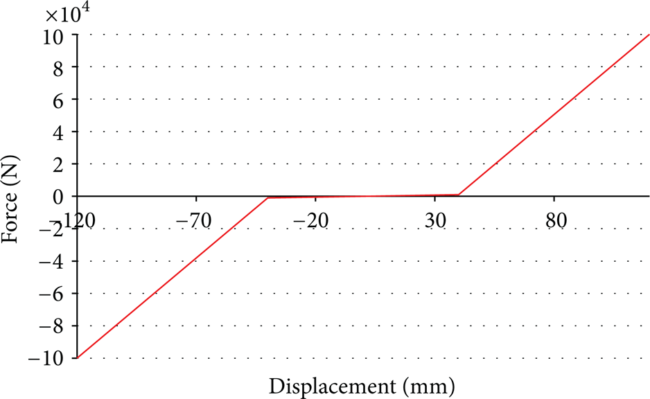
Force-displacement curve for the nonlinear springs.

Figure 6:

Fifth wheel model with one spring.

The main disadvantages of this model, are that the geometry of the fifth wheel plate is different from the real one and that the swaying angle (“X”) is ±15° instead of ±5°. Moreover it is a quite complex and noncompact model needs high numerical requirements.

The main advantages are that allows to simulate “Y” and “Z” and the suspensions of the cabin, and that it allows to simulate the real contact between the king-pin sheet and the fifth wheel in a higher area, like it really occurs.

2.3. Fifth Wheel Model with One Spring

This is the last and most accurate fifth wheel model, in which, the real geometry of a fifth wheel plate has been used. The model has the same joints between the king-pin and the fifth wheel using MPCs like in the previous model and a contact between the rigid fifth wheel plate (with a new geometry) and the king-pin sheet.

Two hinge connectors have been used, one after the other, which allow only a relative rotation in one direction defined by two nodes, to simulate the ±15° and the ±5° rotations, so that the swaying and the pitch can be simulated. To model the ±15° and ±5° stop angles, one stop condition has been used for each hinge.

After the second connector, a spring has been located (like in the previous model) that simulates the tractor unit suspension. Then, a quite accurate and compact fifth wheel model has been obtained, with the same rotations as the real vehicle allowed and with the suspension included.

The main disadvantages of this model, as in the previous one, are the necessity of carrying out a nonlinear analysis with a higher numerical complexity and that the fifth wheel elements used increase the numerical complexity of the analysis and the CPU time; like in the previous model.

Figure 7 shows the fifth wheel model and a sketch of it.

Figure 7:

Quarter vehicle model for a suspension.

3. Suspension Simulation

Another part of the vehicle that must be adequately characterized in order to achieve a good accuracy with the real results is the suspension of the vehicle, so, in this chapter, some different numerical models have been described. There have been models made for the most common types of suspension [5]: the mechanical one (used usually for public works) and pneumatic one (for the rest of the applications). So, although suspensions for three-axis semitrailers will be analyzed, they can also be used for two-axis ones easily.

Any suspension system is usually composed of an elastic element, in parallel a dumping element, and the wheels system, which can be simulated like another in parallel system with a spring and a dumping. So, for a wheel, the next figure quarter vehicle model simulates its static and dynamical behaviour [6, 7].

For Figure 8:

K_s is the suspension stiffness coefficient,

K_ns is the wheel stiffness coefficient,

c_s is the dump coefficient of the dumping,

c_ns is the dump coefficient of the wheel,

m_ns is the nonhanged mass: axis, pneumatic, rim, and so forth.

Figure 8:

Middle vehicle model for a suspension.

It must be highlighted that the dumps do not act during a static load case, so they can be erased in the model, but they must be included for dynamic load cases. Figure 8 shows a middle vehicle model, and there are also full vehicle models [8].

The full vehicle model for a semitrailer will include the same number of middle vehicle models tan number of axes that it has. To simulate the axes in the vehicles, each one is going to be modeled like a bar located between the centers of each wheel with an equivalent rigidity. Then, wheels are modeled like a spring because load cases usually used to analyze a vehicle are static load cases, so the effects of their dumping can be erased, so they can be modeled like a spring, with the rigidity of the wheel (Figure 9) and a nonhanged mass, with the mass of the wheel and the rim. The rigidity of the rim is too high compared with the rigidity of the wheel; therefore it can be omitted [9].

Figure 9:

Wheel model and rigidity curve of a semitrailer wheel depending on the internal pressure (bar).

3.1. Mechanical Suspension

Quite robust mechanical suspensions are usually installed in public works semitrailers because they have a good behaviour in adverse work conditions (gravel deposits, quarries, tacks, etc.), showing a good reliability and a low mechanical wear-out compared with other pneumatic suspensions. Nevertheless they have a worse dynamic behavior, so the comfort and the adaptation of the suspension to the ground are worse too.

These suspensions have usually a mechanical spring that acts elastically, a dumping element, the elements to join the spring to the crossbar of the vehicle, the axis, and the wheel with the rim, as Figure 10 shows.

Figure 10:

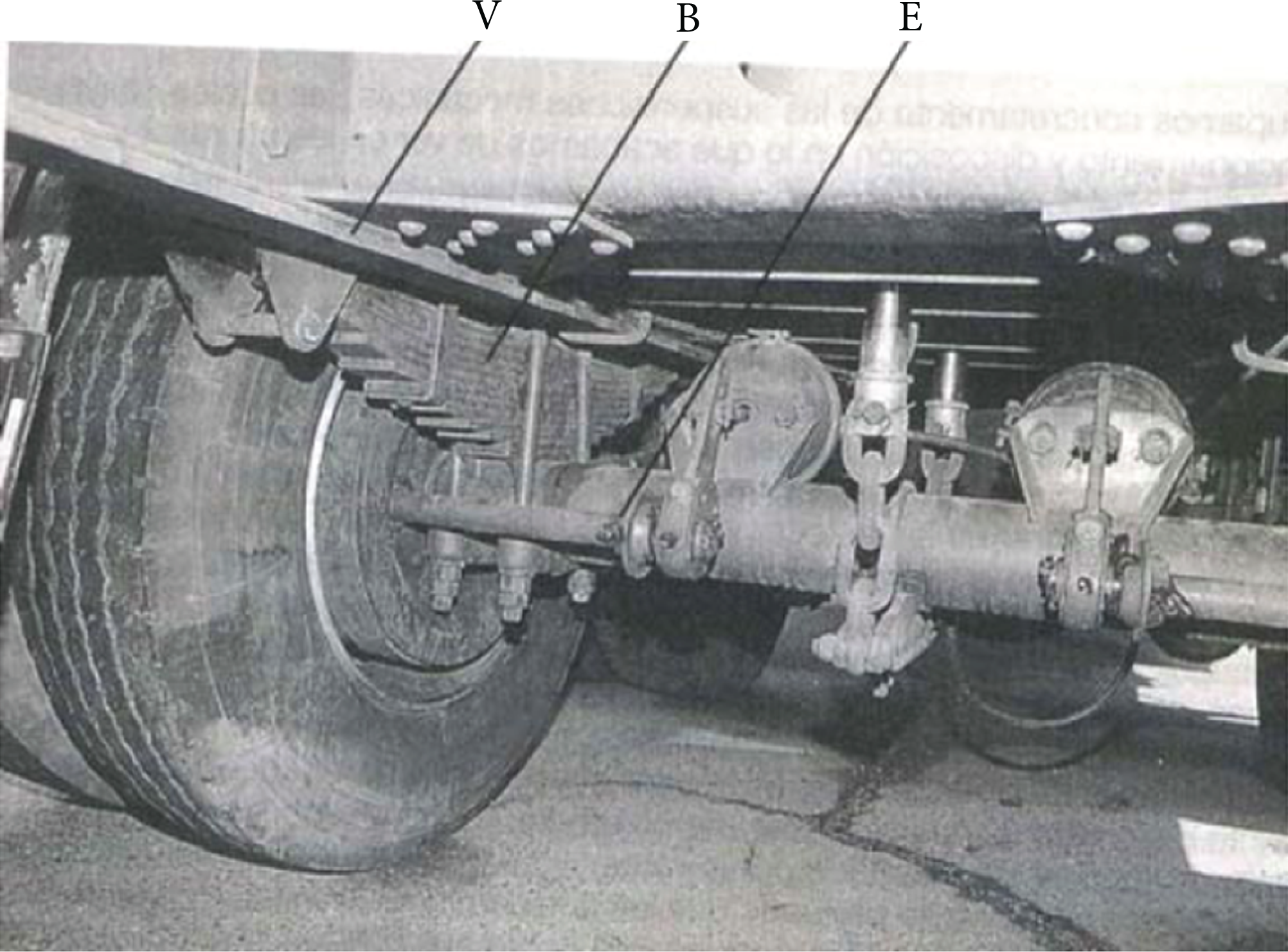
Mechanical suspension with spring (B), crossbars (V), and axis (E).

As we can see in Figure 11, there are two different types of springs: conventional and parabolic ones, but parabolic springs are not used in heavy vehicles. They will be simulated both like a spring with the equivalent elastic coefficient.

Figure 11:

Conventional (a) and parabolic spring (b).

There are other types of suspensions, for instance, the double spring suspension (Figure 12), in which, depending on the payload of the vehicle, only one spring acts (low loads and less rigid suspension) or both springs act together (high loads and more rigid suspension).

Figure 12:

Double-spring suspension: secondary spring (1), main spring (2), U bolts (3), secondary spring support (4), and crossbar of the vehicle (5).

In any suspension system, springs are as important as the joint systems because they allow certain displacements and rotations that keep them working in order. For these springs, one end is fully clamped, except for the transversal rotation (see Figure 13), and the other end allows all the displacements and rotations, except for the longitudinal displacement and the transversal rotation; to achieve this behaviour two different types of joints are possible, corresponding to springs with housings and to friction springs, which define two types of mechanical suspensions.

Figure 13:

spring with housings (a) and friction spring (b).

Concerning the suspension configurations for a semitrailer, there are several different configurations: individual, with one bogie, with two bogies, and so forth. Here, only the individual configuration has been taken into consideration, but results can easily be extrapolated to other models. Three types of mechanical suspensions have been developed.

To obtain the spring behaviour of the suspension, an experimental analysis with a real vehicle has been carried out (Figure 14).

Figure 14:

Experimental results for a real suspension.

Model 1. This model is used with the fifth wheel model 1 because although it is a model that clamps the supports of the suspensions (see Figure 15), nonreal stress concentration zones with appearing near these parts, it can be used to simulate and to model the behaviour of the elements that are far from these zones. It can also be used to obtain the maximum deformation of the vehicle but not the maximum displacement because it does not include the rigidity of the suspension. The main advantages of this model are its simplicity and its lower numerical complexity.

Figure 15:

Suspension model with all the suspension supports clamped.

Model 2. In this model, showed in Figure 16, the suspension is simulated with a rigid bar element, which joins the support zones of the real spring, allowing only the transversal rotation (using a hinge connector, point red in Figure 16) in one of the ends, and, on the other, there is a hinge connector (red) with cylindrical connector before it (two green points) for the friction spring (a), or, for a spring with housings (b), there are a hinge and, after it, a rigid bar (blue), and another hinge connector. These models allow to simulate the behavior of the ends of the suspension [9]. The rigidity of the suspension is modeled using a spring element, located in the longitudinal position of the wheel, with the equivalent rigidity of the spring and the wheel, obtained using:

\frac{1}{K_{spring_eq}} = \frac{1}{K_{spring}} + \frac{1}{K_{wheel}} .

(1)

The main advantages are that it allows the simulation of all the displacements, rotations, and the vertical rigidity of the suspension system and that it is quite compact and simple to implement. The main disadvantage is that it does not include neither the weight of the axes and the wheels nor their transversal rigidity that is necessary for nonsymmetric load cases such as the case of step in only one wheel.

Figure 16:

Suspension models for a spring with housings (b) and for a friction spring (a).

Model 3. This is the most advanced mechanical suspension model developed and allows simulating the lateral and vertical behavior of the suspension, which is especially important for the analysis of nonsymmetric load cases.

The simulation of the spring is quite similar to the previous model, with the same two different modelizations for the end of the spring. For this model, the spring can be simulated as in model 2, but with some rigid elements and with a spring (Figure 17 right), which does not take in consideration the transversal rigidity of the system, with volumetric elements (Figure 17 middle), which includes lateral and vertical rigidity but implies a higher numerical complexity, and with bar elements (Figure 17 left) where the rigidity of the bars is the same (transversal and vertical) as in the volumetric model and implies a lower numerical cost and complexity.

Figure 17:

Some models of the spring for a double spring suspension.

Figure 17 shows models for a double spring suspension, so, for obtaining a simple one, we only must erase the secondary spring. The simulation the real behaviour of the double suspension, not only of the simulation of both springs and the support of the secondary suspension, is necessary but also a contact between the support and the secondary spring must be used. Furthermore, in a nonloaded state, there must be a space between the secondary spring and the support that really exists in the vehicle (see Figure 17).

To simulate the axis a bar with similar rigidity and mass has been used, and in the joints to the wheel a punctual mass has been included (blue in Figures 18 and 19) to simulate the masses of the rim and the wheel.

Figure 18:

Model for a friction spring.

Figure 19:

Model for a spring with housings.

Figures 18 and 19 show the models used for a friction spring model and for a spring with housings, considering a double spring model.

In Figures 18 and 19, the black bars are rigid bars, the red points are hinge MPCs that allow a transversal rotation, the springs are spring elements to simulate the rigidity of the main and the secondary spring elements and the wheel, blue points are mass elements to simulate the mass of the wheel and the rim, two green points are cylindrical MPCs, the purple bar is a bar with the mass and the rigidity of the axis, and the pink bar is a rigid bar. In those cases where there is a simple spring, the elements of the secondary spring will be erased. If there is a load case where the secondary spring does not act, it can be erased too, but this is not usual during the design process.

This model allows to simulate any type of mechanical suspension and can be adapted to any type of vehicle modifying the dimensions, the masses, and the elastic coefficient of each spring; moreover the suspensions are simulated with their transversal and vertical rigidity and with all the nonhanged masses.

The main disadvantages of this model are its complex implementation including some connectors, springs, and masses and the fact that, for the double spring suspension, there is a contact (so nonlinear analysis must be made) that must be included, which could lead to some convergence problems. This entails that both the numerical requirements and the time necessary to converge increase.

Complete Suspension Models. Another aspect to take into consideration for the suspension systems is that for tandem suspensions, each wheel must support the same load. To simulate this requirement, some joints must be included in the suspensions as well as other auxiliary elements for joining some springs. Figure 20 shows a simplified tandem suspension, using the second suspension model described before.

Figure 20:

Second suspension model for a mechanical tandem suspension.

If a force equilibrium analysis is made, it can be observed that the vertical load for each wheel is the same. This tandem model can be easily extrapolated to the third mechanical suspension model.

3.2. Pneumatic Suspension

This is the most common suspension system for semitrailers; therefore it must be perfectly simulated. The first step has been the analysis of the elements and components comprising it and their behavior. These elements are shown in Figure 21 [10], and for the simulation process, only the diapress (element 11; see Figure 22) and the spring (element 7; see Figure 22) have been considered important; the other elements are used for assembly purposes between the parts.

Figure 21:

Pneumatic suspension.

Figure 22:

Sketch and a photo of a diapress.

The spring of the pneumatic suspension is quite similar to the mechanical one; there is only one because one of the ends is joined to a diapress, so previous spring models can be used.

The diapress is a part that joins the spring to the cross-bar of the vehicle, and it is an air cushion with a constant area that only can transmit vertical forces between their ends [11]. It is connected to the other diapresses of the vehicle and to the air compressor of the tractor unit by a pneumatic circuit, so the force transmitted by each of the diapresses is the same because they have the same pressure and the same vertical area. There is another element, the levelling valve (see Figure 23), which is joined to the chassis and to one of the axis (usually the central one for three-axis vehicles and the rear one for two-axis ones).

Figure 23:

Levelling valve and its location.

This valve, depending on the distance between the axis and the chassis, allows the air flow to the diapresses when the distance is lower than the reference one; by this way the pressure inside the diapresses increases and the suspension tends to rise in order to reach the reference level in the levelling valve [12]. If the distance in the levelling valve is lower than the reference one, the valve allows the air inside the diapresses to escape to the atmosphere, so the pressure inside the diapresses is reduced as well as their height, until the levelling valve reaches its reference level. There is a margin for the reference level value that allows the valve not to be constantly working.

We have pointed out that the pressure, the area, and so the forces in the diapresses are the same for all, so if we make a force equilibrium analysis, we obtain that the vertical force for each wheel is the same, like in a tandem model.

In this paper, some models for the pneumatic suspension have been developed. Model 1 is like the mechanical suspension model 1.

Model 2. In this model the diapresses and the springs are simulated like springs, one with a nonlinear behaviour and the other with a linear one, as shown in Figures 24 and 25.

Figure 24:

Pneumatic suspension second model.

Figure 25:

Rigidity coefficient curve for the nonlinear spring to simulate the diapress.

The spring that simulates the spring element has a linear behavior with the rigidity coefficient (K₁) of this element, and the spring that simulates the diapress has a nonlinear force-displacement curve (K₂) which is presented in Figure 25.

With this curve, all the diapress has the same vertical force that must be previously calculated to adapt the curve to obtain this value, and there is a flat zone where the force value is quite similar for different displacements [13].

In order to simulate the lateral and transversal behaviour of the diapress, only the vertical displacement has been clamped.

This is a quite easy model, and if we obtain previously the force acting at each diapress and adjust the curve of the diapress, its vertical behavior is reproduced quite similarly. With this model, although we can obtain the local stresses near the suspensions and the vertical displacement with a low accuracy level, it shows low convergence problems and a low numerical complexity. Its main problem is due to the fact that the model needs a previous calculation to obtain the diapress curve, and additionally it does not consider the nonhanged masses, the axis, the levelling valve, or the wheel rigidity. Another problem is that the behavior of the spring depends on the pressure of the diapress, and it cannot be used for nonsymmetric load cases.

Model 3. The previous model has some errors and disadvantages that must be corrected; therefore the suspension simulation has been improved with a new model. To simulate the behavior of the levelling valve and its influence on the pressure of the diapresses, it has been necessary to use an ABAQUS subroutine. The other elements: the axis, the wheel, and the spring can be simulated without a subroutine, similarly as in the mechanical suspension models. So to simulate the behavior of the levelling valve, it is necessary to use two additional nodes: one is located in the axis and the other in the chassis zone where the levelling valve is located. These nodes can be joined together with some bars that will not be affected by loads.

The key for a good simulation process is the subroutine performance that must read from the results file (.odb) the global position of both nodes, obtain the global distance between them, and then compare this distance with a previous established range of distances. If the distance read is higher, the subroutine must reduce the pressure applied to the diapresses to decrease the distance to the range values, and if it is lower, it must increase it.

Moreover, during the first time increment, it must apply a pressure to each end of the diapresses, obtained as the force obtained in Figure 25 divided by the area of the diapresses.

The diapresses must not be modeled, but there must be selected several zones of the chassis, with their same area, and the pressure must be applied in these locations. The same occurs for the end of the spring in contact with the diapress that must be simulated like a sheet with a high rigidity joined to the end of the spring and where we apply the pressure of the subroutine (see Figure 26).

Figure 26:

Main dimensions of the vehicle.

Concerning the subroutine, there have been used two different subroutines joined with global variables: one to obtain the relative distance between the nodes at the ends of the levelling valve and another, after obtaining the pressure, to apply it to the ends of the diapresses.

The first one is a URDFIL ABAQUS subroutine that reads the results file (.odb) in each time increment and must, for the zero increment, read the distance between the levelling valve nodes (introducing their node numbers in the subroutine), obtain the relative distance, and archive it as a reference value (d₀); the distance range will be: $[d_{0} - R / 2, d_{0} + R / 2]$ , where R is the range of the levelling valve in mm (usually 20 mm) and must be provided to the subroutine.

The function used to obtain the pressure is

P_{ref} = \frac{w_{veh} + w_{load}}{f \cdot A_{diap}},

(2)

F = \frac{L_{vehi}}{L_{vehi} - a / 2 + b},

(3)

P (increment = 1) = P_{ref} \cdot \frac{t_{1}}{t_{tot}},

(4)

P (increment = n \neq 1) = P (n - 1) - K (d_{t} - d_{0}) \cdot \frac{t_{n}}{t_{tot}} if d_{t} \notin [d_{0} - \frac{R}{2}, d_{0} + \frac{R}{2}],

(5)

P (increment = n \neq 1) = P (n - 1) \cdot \frac{t_{n}}{t_{tot}} if d_{t} ε [d_{0} - \frac{R}{2}, d_{0} + \frac{R}{2}],

(6)

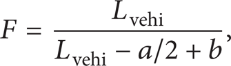
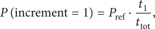
where w_veh is the empty weight of the vehicle, w_load is the payload, n is the increment, t is the total time of the increment, A_diap is the transversal area of the diapress, and K is a convergence constant (it has been used 1.1).

The pressure will be applied with a DLOAD subroutine to the specified elements.

This suspension model allows a perfect simulation of the pneumatic suspension for any static load case; therefore it is specially designed for standard load cases. For dynamic load cases the subroutine will be quite similar, but in these cases the ABAQUS subroutine used to apply the pressure will be a VLOAD subroutine and to read the results a VURDFIL one.

The main disadvantages of this suspension model are that it requires the use of a subroutine which entails a considerable increase of the numerical complexity and the numerical requirements of the analysis and also that the time increment must be quite small to obtain a good convergence of the model, so the time needed to run the analysis increases.

Figure 27 shows a numerical simulation of a tanker vehicle with the suspension model 3. The zones used to apply the pressure can be observed in this figure.

Figure 27:

Model 3 for a pneumatic suspension.

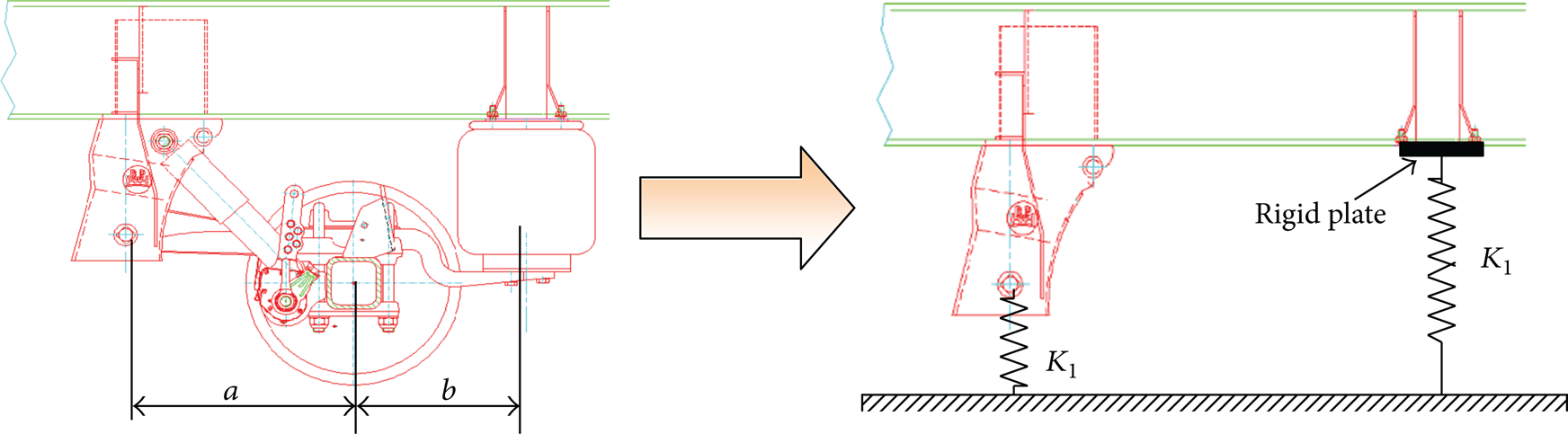
Model 4. Model 3 has the highest accuracy but has some disadvantages as previously indicated, so it has been made another pneumatic model, where some accuracy has been sacrificed to obtain a better convergence as well as lower numerical requirements and calculation time; a subroutine has not been used in model 4. It has been used a nonlinear spring to simulate the suspension as in model 2 (see Figure 25); then, the rigidity of the spring in the flat zone must be obtained previously, with the weight distribution (see Figure 26 and (2) and (3)) and the distribution of weight inside the suspension shared between the diapress and the spring support (see Figure 28 and (7)).

Figure 28:

Force equilibrium equations for a pneumatic suspension.

With a force equilibrium calculation we obtain

F_{spring,plane} = \frac{N_{wheel} \cdot l_{sop}}{l_{sop} + l_{diap}},

(7)

so N_wheel, l_sop, and l_diap, the vertical forces, will be the same for all the axes, and their value will depend on the load level.

Figure 29 shows this numerical model, which is quite similar to the third mechanical suspensión model but with an additional spring to simulate the diapress. SLIDE-PLANE connectors have been used in the diapress end, which restricts all the displacements and all the rotations between their ends in a plane, so the diapress spring only supports vertical forces [9].

Figure 29:

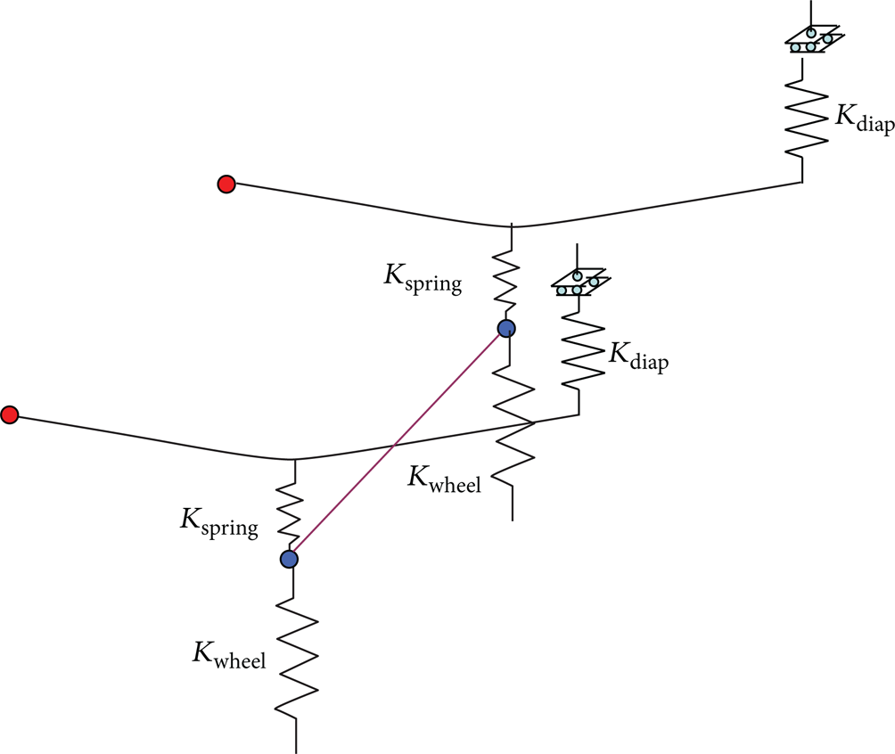
Pneumatic suspension model 4.

The main disadvantages of this model are that it is necessary to obtain previously the vertical forces on each wheel to introduce the nonlinear curve for the diapress and that it uses some connectors and springs, which implies a worse convergence and a higher calculation time but in any case better and smaller than for third model.

The main advantages are that the vertical and transversal rigidity of the suspension can be simulated with a high accuracy, that it is not as difficult to implement as model 3, and that it has better convergence and lower convergence problems than the previous model.

4. Torsion Bar Model

Mechanical suspensions sometimes mount some additional parts, called torsion bars (See Figures 30 and 31) that act when a relative vertical distance appears between the two wheels of an axis, and then they apply a torsion moment to reduce this displacement and avoid that a wheel has an excessive jump.

Figure 30:

Torsion bar.

Figure 31:

Torsion bar location.

The developed model for the torsion bar can be used with the third mechanical suspension model, and it has three bars with the same geometry than a real bar, joined to the extremes of the chassis and to the axis allowing the transversal rotations with hinge connectors, so it must be included to simulate the additional torsion moment that is introduced in the model for some load case, like the step in one wheel load case. In other load cases where a relative vertical displacement does not appear between the wheels of an axis, it does not act, so it is not necessary to include it because its use would imply some additional freedom degrees, convergence problems, and higher modelling complexity [14].

5. Comparative Analysis of the Suspension and the Fifth Wheel Models

To do the comparative analysis, a vehicle tanker has been used where all the mechanical and pneumatic suspensions models and their corresponding fifth wheel model have been placed for a static load case: the rest case with the maximum vehicle payload transported [15, 16].

Results have been analyzed in some parts of the structure, obtaining the stresses (Von Mises), the maximum deformation (see Figure 35), and the vertical displacement. The calculation time required has also been analyzed. It must be pointed out that a plastic material model has been used for all the models, and this implies that a nonlinear analysis must be applied to all of them. Figure 32 shows some of the points used to compare the stresses between the different models.

Figure 32:

Measure points to compare the obtained results.

Analyzing the obtained results (see Figures 32, 33, and 34 and Table 1), the pneumatic suspension models 2, 3, and 4 have the same behavior with similar stresses, displacements, and deformations, so all the models have the same accuracy, but it must be pointed out that model 3 needs higher numerical requirements and CPU time (double the time) to solve the same vehicle, but the accuracy is the same, and it needs to use subroutines; models 2 and 4 need more or less the same CPU time and have the same accuracy, but model 4 includes the axis, the nonhanging mass, and the transversal rigidity, so this model is more adequate for nonsymmetric load cases.

Table 1:

Results for each model.

Suspension model	Fifth wheel model	Maximum deformation	Vertical displacement	Von Mises stress (MPa)								CPU time (s)
Suspension model	Fifth wheel model	(mm)	(mm)	Point 1	Point 2	Point 3	Point 4	Point 5	Point 6	Point 7	Point 8	CPU time (s)

Pneumatic/Mechanic 1	Model 1	10,7	10,7	25,4	73,19	22,06	30,7	69,3	12,9	16,6	23,13	48273
Pneumatic 2	Model 2	11,2	81,8	24,1	57,34	9,4	29,9	250	15,2	8,7	22,73	76454
Pneumatic 2	Model 3	11,4	82,2	24,3	59,2	9,4	31,1	247	15,3	8,9	22,4	73434
Pneumatic 3	Model 3	11,3	81,5	24	58,4	9,5	30,4	248	15,1	8,8	22,5	136567
Pneumatic 4	Model 3	11,2	84,2	24,2	59,6	9,4	31,1	249	15,2	8,7	22,4	84657
Mechanic 2	Model 3	10,6	67,4	26,7	67,5	9,8	33,2	261,1	16,4	8,5	22,3	72453
Mechanic 3	Model 3	10,7	71,3	26,9	66,8	9,7	33,3	260,9	16,5	8,4	22,3	90538

Figure 33:

Von Mises Stress (MPa) for suspension model 1 (a) and for pneumatic model 2 (b).

Figure 34:

Von Mises Stress (MPa) for suspension model 1 (a) and for pneumatic model 2 (b). Details of the king-pin zone and the supports zone.

Figure 35:

Vertical displacements (mm) for suspension model 1 (a) and for pneumatic model 2 (b).

Concerning the mechanical suspensions, models 2 and 3 have the same values in terms of stresses, displacements, and deformations, but they are different from the pneumatic suspension results because they have different vertical rigidity. In this case, model 2 needs a lower CPU time, but, like the pneumatic second model, it is not adequate for nonsymmetric load cases because it does not present a good transversal rigidity behaviour.

The fifth wheel models have been compared with the second pneumatic suspension model and the results show that both models have the same behavior, so all models have the same accuracy, but model 3 needs less CPU time, and it is more compact, and the geometry of the fifth wheel plate is identical to a real one. Therefore model 3 is the best option to simulate this element.

Finally, about the clamped suspension and fifth wheel models (model 1 for both), it can be observed that results in the zones near the clamps (see Figure 33 and Table 1) are different from the other models, so they cannot be used to analyze these zones. In the rest of the zones results are quite similar, so they can be used to analyze and optimize these zones with a lower computational cost. They can also be used to obtain the deformation, not to obtain the vertical displacement, because they do not include the suspension behaviour.

6. Conclusions

The main conclusions are that, with the developed models of fifth wheels and suspensions, the boundary conditions to analyze structurally a semitrailer vehicle can be simulated without the necessity of simulating these elements in detail as indicated by other authors [17]. To make this possible, some different mechanical and pneumatic suspensions and fifth wheel models have been developed, and their behaviour has been compared in terms of stiffness and strength. It can be concluded that the most adequate models are the third mechanical suspension model, the third fifth wheel model, and the fourth pneumatic suspension model if we analyze the accuracy, the computational and CPU cost, and their transversal rigidity behaviour to simulate nonsymmetric load cases.

Footnotes

Acknowledgments

The publication of this research paper has been possible thanks to the funding given by the Industry and Innovation Department of the Government of Aragon as well as by the European Social Funds and to the Research Group GEDiX, according to Regulation (CE) no. 1828/2006 of the 8th of December Commission.

References

Larrodé

Miravete

, and Castejon

, “Design and optimisation of a light-weight frigorific semitrailer,” Heavy Vehicle Systems, vol. 5, no. 1, pp. 45–68, 1998.

and Li

, “A contact finite element algorithm for the multileaf spring of vehicle suspension systems,” Proceedings of the Institution of Mechanical Engineers D, vol. 218, no. 3, pp. 305–314, 2004.

Klemenc

Jurejevcic

, and Fajdiga

, “Fifth wheel,” in Proceedings of the 5th International Design Conference, pp. 19–22, Dubrovnik, Croatia, MAY 1998.

Reboh

Griza

Reguly

, and Strohaecker

T. R.

, “Failure analysis of fifth wheel coupling system,” Engineering Failure Analysis, vol. 15, no. 4, pp. 332–338, 2008.

Bohnett

B. L.

and Bohnett

P. M.

, Fifth wheel travel trailers for example, towing vehicle, support leg manipulating method, involves disengaging support leg locking pin via rod including pin engagement end and handling end.

T.-T.

and Cebon

, “Analysis of a truck suspension database,” Heavy Vehicle Systems, vol. 9, no. 4, pp. 281–297, 2002.

Luque

and Mántaras

D. A.

, “Pneumatic suspensions in semitrailers: part I. General considerations and simplified models,” Heavy Vehicle Systems, vol. 10, no. 4, pp. 295–308, 2003.

ALBA

, Introductión Al Estudio De La Dinámica Del Automóvil, Universidad de Zaragoza, 2001.

Cao

Khajepour

, and Song

, “Modeling and analysis of flexible-wheel suspension concept,” in ASME International Design Engineering Technical Conferences and Computers and Information in Engineering Conference (DETC '09), pp. 921–929, September 2009.

10.

Sujatha

and Tejesu

, “Heavy vehicle dynamics-comparison between leaf spring and hydropneumatic suspensions,” in Proceedings of the 20th Conference on Structural Society of Photo-Optical Instrumentation Engineers (Spie '02), vol. 4753, pp. 311–317, Los Angeles, Calif, USA, 2002.

11.

Luque

and Mántaras

D. A.

, “Pneumatic suspensions in semitrailers: part II. Computer simulation,” Heavy Vehicle Systems, vol. 10, no. 4, pp. 309–320, 2003.

12.

Roebuck

R. L.

Cebon

Jeppesen

B. P.

, and Hague

, “A systems approach to controlled heavy vehicle suspensions,” International Journal of Heavy Vehicle Systems, vol. 12, no. 3, pp. 169–192, 2005.

13.

Richard

M. J.

Bouazara

Khadir

, and Cai

G. Q.

, “Structural optimization algorithm for vehicle suspensions,” Transactions of the Canadian Society for Mechanical Engineering, vol. 35, no. 1, pp. 1–17, 2011.

14.

Lee

and Yang

C. H.

, “An analytical approach for design and performance evaluation of torsion beam rear suspension,” Finite Elements in Analysis and Design, vol. 63, pp. 98–106, 2013.

15.

Cole

D. J.

and Cebon

, “Validation of an articulated vehicle simulation,” Vehicle System Dynamics, vol. 21, no. 4, pp. 197–223, 1992.

16.

Henry

O. L.

, “Design application and comparative tests of trailer air suspension systems,” SAE Transactions, vol. 75, p. 81, 1967.

17.

Egbert

D. E.

and Linlecki

, “Computer optimization of trailer suspensions,” Mechanism and Machine Theory, vol. 16, no. 4, pp. 369–384, 1981.