Sage Journals: Discover world-class research

Abstract

This paper presents a new method to calibrate the robot visual measurement system. In the paper, a laser tracker is used to calibrate the robot twist angles. Each axis of the robot is moved to many positions and the positions measured by the laser tracker fit a plane. The normal vectors of the planes are the directions of the Z axes. According to the definition of the robot kinematics model parameters, the errors of the twist angles can be calculated. The joint angles zero offsets are calibrated by the constraint that the rotation relationship between the world frame and the robot base frame is relatively constant. A planar target with several parallel lines is used to obtain the pose of the camera relative to the planar target by the lines in the target plane and the vanishing line of the plane. The quantum behaved particle swarm optimization (QPSO) algorithm is used to calculate the parameters. Experiments are performed and the results show that the accuracy of the robot visual measurement system is improved about 10 times after being calibrated.

1. Introduction

3D surface topography measurement and the aiming and positioning of the butt joint are key technology in large scale equipment manufacture and assemble process. With the developing of computer vision technology, visual measurement system as a kind of noncontact measurement method is used more and more widely. Besides noncontact, it has the advantages of high measuring precision and measuring speed. When the tested objects have fixed testing characteristics, or are mass produced, the framework structure is used. But, with the increase of the structure complexity and high machining precision requirement of mechanical parts, the demand to measuring is more and more strict. The framework structure cannot meet the measuring requirement. A flexible measurement system which can measure any part of the tested object is needed. Robot visual measurement system is a combination of robot and visual measurement system. Robot vision is seen to be the most important sensory ability for the robot [1]. Cameras fixed on the robot arm allow it not only to have the robot advantages of large flexible global motion but also to have the advantages of the visual measurement system.

Generally, industrial robots have high repeatability but low absolute accuracy, and the characteristic of the robot makes robot visual measurement systems cannot meet the requirement in some situations. Therefore, it is important to improve the absolute accuracy to enhance the measuring accuracy of robot visual measurement systems. Five error sources are known to lead to robot inaccuracy, such as errors in geometrical parameters, environment, measurement, calculation, and use. The geometrical parameter errors are the dominant error source which account for 90% of the errors [2]. So it is important to identify the geometrical parameter errors. There are a lot of researches about robot calibration [3 –10], and most of them are based on the distance constraint. On this occasion, although the robot kinematical parameters are calibrated, the results are inaccurate without using the rotation constraint sufficiently. In the paper, the rotation constraint is introduced. The pose of the world frame relative to the camera frame can be obtained by a planar target with parallel lines using the features of the vanishing points and vanishing lines.

For the robot visual measurement system, it is important to know the relationship between the robot and the camera, which is called the hand-eye calibration. The hand-eye calibration methods are mature [11 –14], and most of them are solved by the equation AX = XB. The rotation is calculated first, and then the translations are attained. So, in the paper, the procedure of calculating the hand-eye relationship is not introduced.

For most conventional optimization methods, for example, least squared algorithm [15], which is based on quadratic error functions, the iterative initial values have a great contribution to the results. That means that the optimization results are not the global optimum while they are just the approximate extreme points in the solution space. Now that the traditional methods cannot deal with nonlinear systems effectively, some new methods drawn from the field of biology are proposed to be the alternation. Genetic algorithms (GA) [16 –19], artificial neural networks [20 –22], and particle swarm optimization algorithm [23, 24] are used to identify parameters to improve the robot accuracy. Hassan et al. [25] had proved that the particle swarm optimization algorithm had better optimization capability than other optimization algorithms. Though the PSO [26] algorithm can solve some problems efficiently, it has disadvantage that it does not guarantee the global optimum [27, 28]. To overcome the shortcoming, the QPSO algorithm is proposed [29]. In the paper, the QPSO algorithm is used to obtain the real joint angles zero offsets.

According to the D-H model, the rotation of the transformation from the robot end effector to the robot base frame is only related to the robot twist angles and joint angles. So the twist angles and the joint angles can be calibrated using the rotation constraint. The errors from twist angles and joint angles have more contributions to the robot accuracy than link lengths and link joint offsets. So the proposed method is a simple way to calibrate robot when the measuring requirement is not too strict.

This paper is organized as follows. The calibration principle will be presented in Section 2. Experiment results will be shown in Section 3, and the conclusion will be provided in Section 4.

2. Calibration Principle

As shown in Figure 1, there is a camera fixed on the robot end effector. The camera frame is denoted by F_c. The world frame is created on the left top corner of the planar target, which has black and white lines on it, and is denoted by F_w. The robot base frame F_r and the world frame F_w are relatively stationary. The camera is moved to different positions with the robot, and the transformations ${T_{c}}^{r}$ and ${T_{w}}^{c}$ are changed at the same time. But the product of the two matrices is constant, where ${T_{w}}^{c}$ is the transformation from the world frame F_w to the camera frame F_c and ${T_{c}}^{r}$ is the transformation from the camera frame F_c to the robot base frame F_r, which is the product of the transformations T₆ and T_h.

Figure 1:

Robot visual measurement system calibration model.

2.1. Calibration of Twist Angles

According to the definition of the kinematical parameters of D-H model, the twist angle describes the angle between two Z axes of the adjacent links. When the robot is given, the twist angles are determinate. So the real Z axes should be determined first to calibrate the twist angles. A laser tracker is used to measure the real Z axes directions of the robot. The reflector is fixed on the robot end effector, and the first axis of the robot is moved in the joint angle range uniformly. The motion curve of the reflector is a spatial circular arc, and the normal vector of the arc plane is the direction of the robot first link Z axis.

Suppose that the positions of the reflector are (x₁ⁱ, y₁ⁱ, z₁ⁱ), where i is the ith position when the first axis is moved. Then, the plane can be written as

a_{1} x_{1}^{i} + b_{1} y_{1}^{i} + c_{1} z_{1}^{i} + d_{1} = 0,

(1)

where v₁ = (a₁, b₁, c₁) is the unit normal vector of the plane fitted by the positions (x₁ⁱ, y₁ⁱ, z₁ⁱ). And it is also the direction of the first link Z axis.

The same operations are performed to the rest links, and the directions of the Z axes are obtained and denoted as v_axis = (a_axis, b_axis, c_axis)(axis = 2, 3, 4, 5, 6).

So the angle between the first and the second links can be obtained as

α = arccos (v_{1} \cdot * v_{2}) .

(2)

The sign can be determined by the definition of the twist angle. Therefore, the real twist angle can be written as

α_{1}^{'} = (sign) α .

(3)

The rest twist angles can be attained as (2) and (3), and the twist angles errors can be obtained as follows:

\begin{matrix} Δ α_{1} = α_{1}^{'} - α_{1}, \\ Δ α_{2} = α_{2}^{'} - α_{2}, \\ Δ α_{3} = α_{3}^{'} - α_{3}, \\ Δ α_{4} = α_{4}^{'} - α_{4}, \\ Δ α_{5} = α_{5}^{'} - α_{5}, \\ Δ α_{6} = α_{6}^{'} - α_{6}, \end{matrix}

(4)

where α_i′, α_i, and Δα_i (i = 1, 2, … 6) are the true value, the ideal value, and the error of the twist angles.

But it is worth noting that there is a link gear between the link 2 and link 3. When the link 2 is moved, the link 3 is moved at the same time. But it is not the same for the reverse condition. So when the operation is performed to the link 2, the reflector should be fixed on the arm of the link 2, rather than on the robot end effector.

2.2. Calibration of Joint Angles

The resolution of the robot axes is about 0.01°, so the errors from the recorders can be ignored. The joint angles errors mentioned there mean errors of the joint angle zero offsets.

The robot base frame F_r and the world frame F_w are relatively stationary. Therefore, there is a constant equation as

{}^{r}{T_{w}} = {}^{r}{T_{c}} * {}^{c}{T_{w}} = T_{6} * T_{h} * {}^{c}{T_{w}},

(5)

where the matrix T_h is the hand-eye relationship transformation, which has been obtained already. The matrices T₆ and ${T_{w}}^{c}$ are variable with the robot moving.

According to (5), we have

{}^{r}{R_{w}} = R_{6} * R_{h} * {}^{c}{R_{w}},

(6)

where ${R_{w}}^{r}$ , R₆, R_h, and ${R_{w}}^{c}$ , are the rotations of the transformations ${T_{w}}^{r}$ , T₆, T_h, and ${T_{w}}^{c}$ .

2.2.1. Solving R₆

The robot is a six-degree-of-freedom serial industrial robot. According to the D-H model, the pose and position of each link can be expressed as (7). The kinematical parameters are shown in Table 1. Consider

\begin{matrix} {}^{r}{T_{1}} = [\begin{bmatrix} c θ_{1} & - c (α_{1} - \frac{π}{2}) * s θ_{1} & s (α_{1} - \frac{π}{2}) * s θ_{1} & a_{1} * c θ_{1} \\ s θ_{1} & c (α_{1} - \frac{π}{2}) * c θ_{1} & - s (α_{1} - \frac{π}{2}) * c θ_{1} & a_{1} * s θ_{1} \\ 0 & s (α_{1} - \frac{π}{2}) & c (α_{1} - \frac{π}{2}) & d_{1} \\ 0 & 0 & 0 & 0 \end{bmatrix}], \\ {}^{1}{T_{2}} = [\begin{bmatrix} c (θ_{2} - \frac{π}{2}) & - c (α_{2}) * s (θ_{2} - \frac{π}{2}) & s (α_{2}) * s (θ_{2} - \frac{π}{2}) & a_{2} * c (θ_{2} - \frac{π}{2}) \\ s (θ_{2} - \frac{π}{2}) & c (α_{2}) * c (θ_{2} - \frac{π}{2}) & - s (α_{2}) * c (θ_{2} - \frac{π}{2}) & a_{2} * s (θ_{2} - \frac{π}{2}) \\ 0 & s (α_{2}) & c (α_{2}) & d_{2} \\ 0 & 0 & 0 & 1 \end{bmatrix}], \\ {}^{2}{T_{3}} = [\begin{bmatrix} c (θ_{3} - θ_{2}) & - c (α_{3} - \frac{π}{2}) * s (θ_{3} - θ_{2}) & s (α_{3} - \frac{π}{2}) * s (θ_{3} - θ_{2}) & a_{3} * c (θ_{3} - θ_{2}) \\ s (θ_{3} - θ_{2}) & c (α_{3} - \frac{π}{2}) * c (θ_{3} - θ_{2}) & - s (α_{3} - \frac{π}{2}) * c (θ_{3} - θ_{2}) & a_{3} * s (θ_{3} - θ_{2}) \\ 0 & s (α_{3} - \frac{π}{2}) & c (α_{3} - \frac{π}{2}) & d_{3} \\ 0 & 0 & 0 & 1 \end{bmatrix}], \\ {}^{3}{T_{4}} = [\begin{bmatrix} c θ_{4} & - c (α_{4} + \frac{π}{2}) * s θ_{4} & s (α_{4} + \frac{π}{2}) * s θ_{4} & a_{4} * c θ_{4} \\ s θ_{4} & c (α_{4} + \frac{π}{2}) * c θ_{4} & - s (α_{4} + \frac{π}{2}) * c θ_{4} & a_{4} * s θ_{4} \\ 0 & s (α_{4} + \frac{π}{2}) & c (α_{4} + \frac{π}{2}) & d_{4} \\ 0 & 0 & 0 & 1 \end{bmatrix}], \\ {}^{4}{T_{5}} = [\begin{bmatrix} c (θ_{5} + π) & - c (α_{5} + \frac{π}{2}) * s (θ_{5} + π) & s (α_{5} + \frac{π}{2}) * s (θ_{5} + π) & a_{5} * c (θ_{5} + π) \\ s (θ_{5} + π) & c (α_{5} + \frac{π}{2}) * c (θ_{5} + π) & - s (α_{5} + \frac{π}{2}) * c (θ_{5} + π) & a_{5} * s (θ_{5} + π) \\ 0 & s (α_{5} + \frac{π}{2}) & c (α_{5} + \frac{π}{2}) & d_{5} \\ 0 & 0 & 0 & 1 \end{bmatrix}], \\ {}^{5}{T_{6}} = [\begin{bmatrix} c θ_{6} & - c α_{6} * s θ_{6} & s α_{6} * s θ_{6} & a_{6} * c θ_{6} \\ s θ_{1} & c α_{6} * c θ_{6} & - s α_{6} * c θ_{6} & a_{6} * s θ_{6} \\ 0 & s α_{6} & c α_{6} & d_{6} \\ 0 & 0 & 0 & 1 \end{bmatrix}], \end{matrix}

(7)

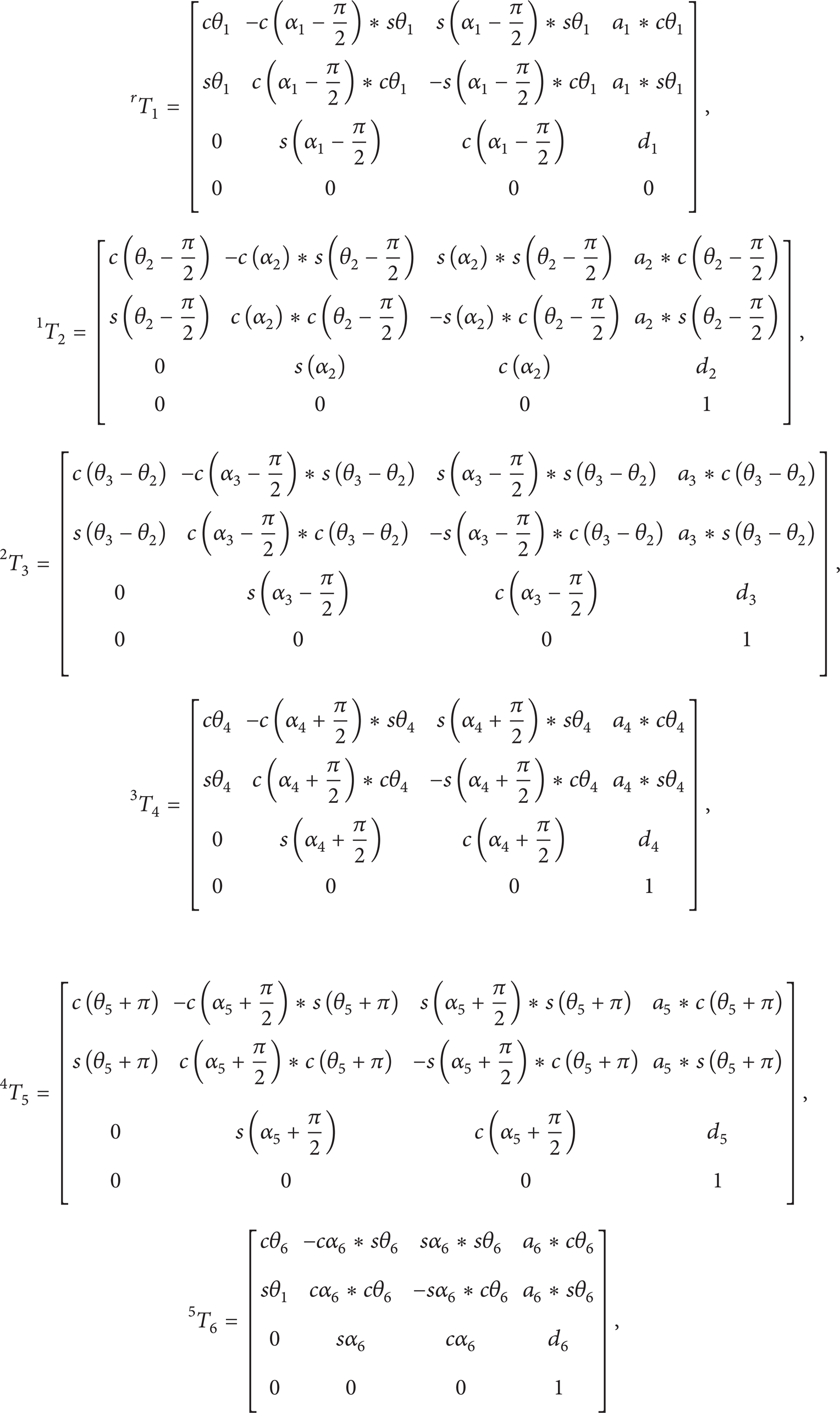
where cθ is the cosine value of the angle θ and sθ is the sine value of the angle θ.

Table 1:

IRB1400 robot kinematical parameters.

No.	Joint angle	Link joint offset	Link length	Link twist
No.	range θ/°	d/mm	a/mm	angle α/°

1	−170∼170	475	150	−90
2	−70∼70	0	600	0
3	−65∼70	0	120	90
4	−150∼170	720	0	−90
5	−115∼115	0	0	90
6	−300∼300	85	0	0

The transformation from the robot end effector to the robot base frame can be written as

T_{6} = {}^{r}{T_{1}} * {}^{1}{T_{2}} * {}^{2}{T_{3}} * {}^{3}{T_{4}} * {}^{4}{T_{5}} * {}^{5}{T_{6}} .

(8)

From (7), we can see that R₆ is only determined by the twist angles α and the joint angles θ.

2.2.2. Solving ${}^{c}{R_{w}}$

The camera is calibrated using the method proposed by Zhang [30].

If there are at least three coplanar equally spaced parallel lines on the scene plane, the ${R_{w}}^{c}$ can be computed according to the properties of the vanishing point and vanishing line [31].

There are a set of parallel lines on the planar target, and the lines are coplanar and equally spaced parallel. Three equally spaced lines on the scene plane are represented as

\begin{matrix} a_{1} x + b_{1} y + c_{1} = 0, \\ a_{2} x + b_{2} y + c_{2} = 0, \\ a_{3} x + b_{3} y + c_{3} = 0 . \end{matrix}

(9)

The vanishing point of the three parallel lines is named as v = (x_v, y_v, 1)^T, which is the intersection point of the three parallel lines.

According to the equation

v = K d,

(10)

the direction of the parallel lines measured in the camera frame can be expressed as

d = \frac{K^{- 1} v}{∥ K^{- 1} v ∥},

(11)

where K are the internal calibration parameters of the camera.

The direction d is the Y axis of the world frame expressed in the camera frame.

The three equally spaced lines on the planar target can be represented as

\begin{matrix} l_{1} = (a_{1}, b_{1}, c_{1}), \\ l_{2} = (a_{2}, b_{2}, c_{2}), \\ l_{3} = (a_{3}, b_{3}, c_{3}) . \end{matrix}

(12)

The solution for the vanishing line is,

l = ({(l_{1} \times l_{3})}^{T} (l_{2} \times l_{3})) l_{2} + 2 ({(l_{1} \times l_{2})}^{T} (l_{3} \times l_{2})) l_{3} .

(13)

According to the equation

l = K^{- T} n,

(14)

the orientation of the target plane can be represented in the camera frame as

n = \frac{K^{T} l}{∥ K^{T} l ∥} .

(15)

The direction n is the Z axis of the world frame expressed in the camera frame.

Then, the direction of X axis of the world frame expressed in the camera frame can be obtained as

X = Y \times Z .

(16)

Therefore, the transformation ${R_{w}}^{c}$ can be represented as

{}^{c}{R_{w}} = [\begin{bmatrix} X & Y & Z \end{bmatrix}] .

(17)

2.2.3. Quantum Behaved Particle Swarm Optimization

Particle swarm optimization (PSO) was first introduced by Kennedy and Eberhart. In the PSO algorithm, every swarm particle explores a possible solution. At first, the initial particles are generated in the searching space randomly. Then, the particles as their personal best positions are used to evaluate the fitness function determined by the optimization problem. And the best position of the whole flock is the global best solution. Then, the swarms adjust their own velocities and positions dynamically based on the personal best positions and global best positions as the following equations:

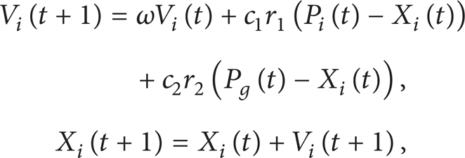
\begin{matrix} V_{i} (t + 1) = ω V_{i} (t) + c_{1} r_{1} (P_{i} (t) - X_{i} (t)) + c_{2} r_{2} (P_{g} (t) - X_{i} (t)), \\ X_{i} (t + 1) = X_{i} (t) + V_{i} (t + 1), \end{matrix}

(18)

where c₁ and c₂ are the acceleration coefficients, ω is the inertia weight factor, r₁ and r₂ are random numbers in the range of (0, 1), X_i(t) is the ith particle, P_i(t) is the personal best position of the ith particle, and P_g(t) is the global best position of the entire population.

Every swarm continuously updates itself through the above mentioned best positions. In this way, the particles tend to reach better and better solutions in the searching space.

In the PSO algorithm, the particles will follow a particular course after several iterations. And then the particles will be trapped into local optima. So the global convergence cannot be guaranteed which has been proved by Bergh. To make sure that the particles escape from a local minimum, the QPSO algorithm is proposed. In the QPSO algorithm, the particle position is described not by the velocity but by the particle's appearing probability density function. There is no fixed orbit for the particles, and the particles constrained by δ potential trough can appear at any position in the feasible solution space with certain probability. So the QPSO can guarantee the global convergence and it has been proved by Sun.

The particle position updating equations are as follows:

\begin{matrix} C_{j} = (C_{1}, C_{2}, \dots, > C_{D}) = \frac{1}{M} \sum_{i = 1}^{M} P_{i} = (\frac{1}{M} \sum_{i = 1}^{M} P_{i, 1}, \frac{1}{M} \sum_{i = 1}^{M} P_{i, 2}, \dots, \frac{1}{M} \sum_{i = 1}^{M} P_{i, D}), \\ p_{i, j} = ϕ \cdot P_{i, j} + (1 - ϕ) \cdot G_{i, j}, \\ x_{i, j} = p_{i, j} \pm α \cdot | C_{j} - x_{i, j} | \cdot \ln [\frac{1}{u}], \end{matrix}

(19)

where ϕ ∼ U(0 ∼ 1), u ∼ U(0 ∼ 1), D is the dimension of the problem space, M is the population size, x_i = (x_i1, x_i2, …, x_iD) are the particle current positions, P_i = (P_{i, 1}, P_{i, 2}, …, P_iD) are the personal best positions, G_i = (G_{i, 1}, G_{i, 2}, …, G_iD) are the global best positions, and α is the Contraction-Expansion coefficient which is the only parameter in the QPSO algorithm depicted as

α = \frac{0.5 * (MAXITER - t)}{MAXITER + 0.5},

(20)

where t is the current iterative number and the MAXITER is the maximum iterative number.

2.2.4. Objective Function

The zero offsets of joint angles need to be computed using the optimization algorithm.

Suppose the true joint angle values are expressed as

\begin{matrix} θ_{1}^{'} = θ_{1} + Δ θ_{1}, \\ θ_{2}^{'} = θ_{2} + Δ θ_{2}, \\ θ_{3}^{'} = θ_{3} + Δ θ_{3}, \\ θ_{4}^{'} = θ_{4} + Δ θ_{4}, \\ θ_{5}^{'} = θ_{5} + Δ θ_{5}, \\ θ_{6}^{'} = θ_{6} + Δ θ_{6}, \end{matrix}

(21)

where θ_i′, θ_i, and Δθ_i (i = 1, 2, … 6) are the true value, the ideal value, and the error of joint angles zero offsets, respectively.

Equations (4) and (21) can be substituted to (7), and the true value R₆′ can be obtained and then can be substituted to (6).

After the robot moved several positions, the objective function is obtained as

F (Δ θ_{1}, Δ θ_{2}, \dots, Δ θ_{6}) = \sum_{i = 1}^{n - 1} \sum_{j = i}^{n} \sum_{k = 1}^{9} {∥ {}^{r}{R_{w}^{i}} (k) - {}^{r}{R_{w}^{j}} (k) ∥}^{2},

(22)

where n is the number of the positions and ${R_{w}^{i}}^{r} (k)$ is the kth element of the rotation matrix at the ith position.

3. Experimental Results

3.1. Experiment Setup

The robot visual measurement system is composed of an industrial robot and a visual measurement system. The visual measurement system consists of a binocular stereo vision system, laser generators, a computer, and the image process system. The robot is an industrial robot IRB1400 from ABB (a Swiss-Swedish conglomerate). The binocular stereo vision system consists of two industrial cameras AVT F504B, with 16 mm lens from Mage. The image resolution of the camera is 2452*2056 pixels. The field of view is about 300*300 mm², and the work distance is about 600 mm. The laser generators are HK130209307-10 from HUAKE. The laser beams produced by laser generators are projected on the tested surface and form light stripes on the surface. The contour of the light stripes is the contour of the test surface, which is simple for measuring.

The two cameras are calibrated using the Zhang [30] method, the left camera frame is the camera frame F_c, and the right camera is an auxiliary camera to measure. The planar gridding target is placed in the robot work space, and the cameras are moved with robot to capture the images of the planar target in different positions.

In the calibrating procedure, a laser tracker and a planar target will be used. The laser tracker is AT901-B from Leica, with the measuring resolution of 0.01 mm. There are parallel lines on the planar target, and the resolution is 5 μm.

The work space of the measuring system is about 1500*1500*1000 mm³. And the system is shown in Figure 2.

Figure 2:

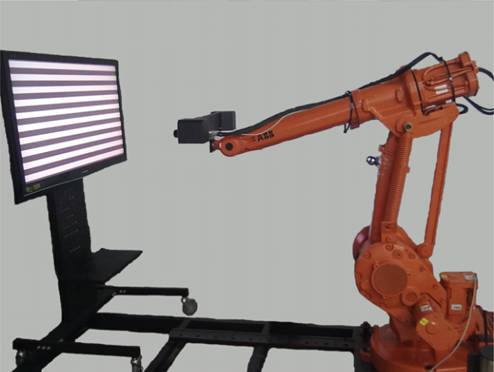
The robot visual measurement system.

3.2. Calibration of Twist Angles

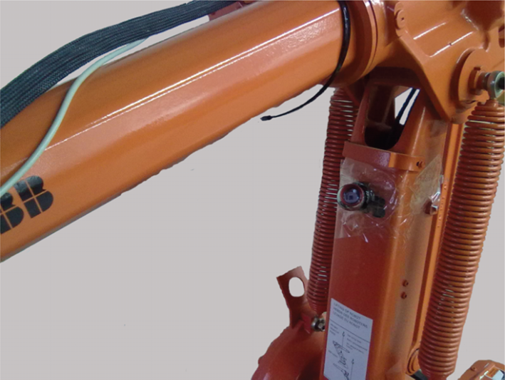
As shown in Figure 3, there is an adapting part fixed on the robot end effector, and the reflector of the laser tracker is fixed on the other end of the adapting part. Each single axis is moved in its joint angle range mentioned in Section 2.1, and 100 pause points are captured uniformly. It is worth noting that, when the axis 2 is moved, the reflector is fixed on the arm of axis 2, as shown in Figure 4. The pause points are measured by the laser tracker, and planes are fitted based on these points. The normal vectors of the planes are the directions of Z axes, and the twist angles are obtained. There are only five twist angles which can be obtained. The last frame is created on the robot end effector, and the sixth twist angle is zero which cannot be calibrated by the method we proposed. The calibration results of the twist angles are shown in Table 2.

Table 2:

The errors of the twist angles.

	Δα₁	Δα₂	Δα₃	Δα₄	Δα₅	Δα₆

Error/rad	0.00059930	−0.00009572	−0.00389624	0.00378916	0.01663513	0

Figure 3:

Adapting part.

Figure 4:

The reflector on the axis 2.

3.3. Solving the Joint Angle Zero Offsets

The camera is moved with the robot to 100 different positions, and at least three parallel lines on the planar target are captured by the left camera. The images are saved and the corresponding joint angles are recorded at the same time. According to Section 2.2.1 and Section 2.2.2, R₆ and ${R_{w}}^{c}$ are computed.

According to the objective functions in Section 2.2.4, the errors of the joint angle zero offsets are computed using the QPSO algorithm.

The particle size is 60, the dimension is 6, the maximum iteration number is 20000, and the range of parameters are (−1, 1). The errors of the joint angle zero offsets are shown in Table 3.

Table 3:

The errors of the joint angle zero offsets.

	Δθ₁	Δθ₂	Δθ₃	Δθ₄	Δθ₅	Δθ₆

Error/rad	0.00029334	−0.00018536	−0.00152726	0.00254384	−0.00709304	0.00004102

3.4. Verified Experiments

To verify the validity of the proposed method, a verified experiment system is set up. The round hole target is put in the robot work space, as shown in Figure 5.

Figure 5:

Verified experiment.

The centers of the holes on the target are measured by the binocular stereo vision system. Then, they can be represented in the robot base frame, by the transformation matrices T₆ and T_h, where the matrix T₆ is obtained by the D-H model with the calibrated parameters α_i′ and θ_i′. At the same time, they are measured using the laser tracker.

Five hole centers measured randomly in the left target and four in the right target have been recorded and the distances of any two hole centers are calculated. Compare the distances measured by the laser tracker and the robot visual measurement system; the results are shown in Table 4.

Table 4:

Verified experiment results.

No.	Laser tracker/mm	Kinematics model/mm	Error/mm	Calibrated/mm	Error/mm

1	1407.3618	1412.3042	4.9424	1407.6420	0.2802
2	1452.8959	1454.6046	1.7087	1453.2856	0.3897
3	1063.4934	1061.4067	−2.0867	1063.2350	−0.2584
4	1456.6879	1456.8733	0.1854	1456.7918	0.1039
5	1316.1796	1314.8049	−1.3747	1315.7760	−0.4036
6	1048.7702	1042.8337	−5.9365	1048.3021	−0.4681
7	1139.2491	1135.6079	−3.6412	1139.0911	−0.1580
8	1273.4407	1268.1671	−5.2736	1273.0968	−0.3439
9	1478.7534	1474.3281	−4.4253	1478.2286	−0.5248
10	1482.4442	1478.8035	−3.6407	1481.8039	−0.6403
11	1078.8065	1077.6482	−1.1583	1078.5412	−0.2653
12	1485.2963	1478.9914	−6.3049	1484.7494	−0.5469
13	1478.5834	1484.2214	5.6380	1478.9045	0.3211
14	1242.6878	1248.9148	6.2270	1243.2032	0.5154
15	1400.1402	1400.0122	−0.1280	1399.8832	−0.2570
16	1070.9431	1070.7926	−0.1505	1070.8120	−0.1311
17	1210.8806	1208.6086	−2.2720	1210.6297	−0.2509
18	1457.8677	1463.4684	5.6007	1458.2994	0.4317
19	1396.1036	1394.2730	−1.8306	1395.7513	−0.3523
20	1479.7462	1474.3030	−5.4432	1478.9971	−0.7491

Mean/mm		0.9682		0.1654
RMS/mm		4.0248		0.4046

From Table 4, we can see that the measuring accuracy is improved after calibration.

4. Conclusion

This paper represents a two-step calibration method for the robot visual measurement system. Firstly, the twist angles are calibrated using a laser tracker. And then, according to the constraint that the world frame and the robot base frame are relatively constant, the joint angles zero offsets are calibrated. The rotation constraint is introduced and the accuracy is improved. The results show that the proposed calibration method in the paper can improve the measuring accuracy greatly. In the calibrating procedure, there are some key problems that need to be noted.

To improve the accuracy, the pause points should be as much as possible when calibrating the twist angles.

In the calibrating procedure, adjust the camera to make sure that the planar target is in the range of the camera depth of field.

The scene plane should be as much lean as possible with the planar target to decrease the effect by the vanishing point position error when calibrating the rotation parameters.

The robot should be moved to cover all the real measuring space to guarantee the measuring accuracy.

The calibration method proposed in the paper has broad applications including numerous other kinds of robot visual measurement systems. After calibration, there is no additional measuring equipment needed in the measuring procedure. The proposed method is simple and easy to perform. It can meet the large scale measurement requirement. But, if the measurement requirement is more restrict, the distance constraint should be used and the link length and link joint offsets should be calibrated. The effects about temperature and elasticity are not discussed either, and the studies on them should be done in the future.

References

Zhong

Qiao

, and Li

, Robot Vision, National Defense Industry Press, 1994.

Judd

R. P.

and Knasinski

A. B.

, “Technique to calibrate industrial robots with experimental verification,” IEEE Transactions on Robotics and Automation, vol. 6, no. 1, pp. 20–30, 1990.

Elatta

A. Y.

P. G.

Fan

L. Z.

, “An overview of robot calibration,” Information Technology Journal, vol. 3, pp. 74–78, 2004.

C. H.

, “The kinematic error model for the design of robot manipulators,” in Proceedings of the American Control Conference, pp. 22–24, San Francisco, Calif, USA, June 1983.

Veitschegger

W. K.

and Wu

C.-H.

, “Robot accuracy analysis based on kinematics,” IEEE Journal of Robotics and Automation, vol. 2, no. 3, pp. 171–179, 1986.

Gatti

and Danieli

, “A practical approach to compensate for geometric errors in measuring arms: application to a six-degree-of-freedom kinematic structure,” Measurement Science and Technology, vol. 19, no. 1, Article ID 015107, 2008.

Chen

Jia

, and Sun

, “Calibration method and experiments of robot kinematics parameters based on error model,” Robot, vol. 34, no. 6, pp. 680–688, 2012.

Wang

Liao

Q.-Z.

Zhuang

Y.-F.

, and Wei

S.-M.

, “Simulation and experimentation for calibration of general 7R serial robots,” Robot, vol. 28, no. 5, pp. 483–494, 2006.

Ren

Y.-J.

Zhu

J.-G.

Yang

X.-Y.

, and Ye

S.-H.

, “Measurement robot calibration model and algorithm based on distance accuracy,” Acta Metrologica Sinica, vol. 29, no. 3, pp. 198–202, 2008.

10.

Wang

, and Wu

, “Novel approach to calibrate main body of a three-dimensional scanning robotic system,” Journal of Mechanical Engineering, vol. 47, no. 17, pp. 9–14, 2011.

11.

Shiu

Y. C.

and Ahmad

, “Calibration of wrist-mounted robotic sensors by solving homogeneous transform equations of the form AX = XB,” IEEE Transactions on Robotics and Automation, vol. 5, no. 1, pp. 16–29, 1989.

12.

Tsai

R. Y.

and Lenz

R. K.

, “New technique for fully autonomous and efficient 3D robotics hand/eye calibration,” IEEE Transactions on Robotics and Automation, vol. 5, no. 3, pp. 345–358, 1989.

13.

Dornaika

and Horaud

, “Simultaneous robot-world and hand-eye calibration,” IEEE Transactions on Robotics and Automation, vol. 14, no. 4, pp. 617–622, 1998.

14.

Yang

G.-L.

Kong

L.-F.

, and Wang

, “A new calibration approach to hand-eye relation of manipulator,” Robot, vol. 28, no. 4, pp. 400–405, 2006.

15.

Nubiola

and Bonev

I. A.

, “Absolute calibration of an ABB IRB 1600 robot using a laser tracker,” Robotics and Computer Integrated Manufacturing, vol. 29, pp. 236–245, 2013.

16.

Parker

J. K.

Khoogar

A. R.

, and Goldberg

D. E.

, “Inverse kinematics of redundant robots using genetic algorithms,” in Proceedings of the IEEE International Conference on Robotics and Automation, pp. 271–276, Scottsdale, Ariz, USA, May 1989.

17.

Tang

and Xu

, “Application of fuzzy Naive Bayes and a real-valued genetic algorithm in identification of fuzzy model,” Information Sciences, vol. 169, no. 3–4, pp. 205–226, 2005.

18.

Chen

J. L.

and Chang

W. D.

, “A multi-crossover genetic algorithm for parameters estimation of a two-link robot,” in Systems Modeling and Simulation, pp. 198–202, Springer, 2007.

19.

Liu

Liang

Qiang

W. Y.

, “Improvement on robots positioning accuracy based on genetic algorithm,” in IMACS Multiconference on Computational Engineering in Systems Applications, pp. 387–392, Beijing, China, October 2006.

20.

Lewis

J. M.

Zhong

X. L.

, and Rea

, “Neural network approach to the robot inverse calibration problem,” in Proceedings of the 2nd International Conference on Intelligent Systems Engineering, pp. 342–347, September 1994.

21.

Zhong

Lewis

J. M.

, and N-Nagy

F. L.

, “Inverse robot calibration using artificial neural networks,” Engineering Applications of Artificial Intelligence, vol. 9, no. 1, pp. 83–93, 1996.

22.

Jang

J. H.

Kim

S. H.

, and Kwak

Y. K.

, “Calibration of geometric and non-geometric errors of an industrial robot,” Robotica, vol. 19, no. 3, pp. 311–321, 2001.

23.

Wang

X. Q.

Liu

H. D.

Shi

Liang

, and Zhang

Y.-C.

, “Research on identification method of kinematics for space robot,” Procedia Engineering, vol. 29, pp. 3381–3386, 2012.

24.

Asgharifard-Sharabiani

Hannaneh

, and Nikkhah-Bahrami

, “Calculation of helical gear's basic parameters using COP-data acquired by optical 3D digitizer,” Proceedings of the Institution of Mechanical Engineers, Part C: Journal of Mechanical Engineering Science, vol. 225, no. 12, pp. 2953–2962, 2011.

25.

Hassan

Cohanim

De Weck

, and Venter

, “A comparison of particle swarm optimization and the genetic algorithm,” in Proceedings of the 46th AIAA/ASME/ASCE/AHS/ASC Structures, Structural Dynamics and Materials Conference, pp. 1138–1150, April 2005.

26.

Kennedy

and Eberhart

, “Particle swarm optimization,” in Proceedings of the IEEE International Conference on Neural Networks, pp. 1942–1948, Perth, Australia, December 1995.

27.

van den Bergh

and Engelbrecht

A. P.

, “A new locally convergent particle swarm optimiser,” in Proceedings of the IEEE International Conference on Systems, Man and Cybernetics, pp. 94–99, October 2002.

28.

Bergh

F. V.

, An analysis of particle swarm optimizers [Ph.D. thesis], University of Pretoria, 2001.

29.

Sun

Feng

, and Xu

, “Particle swarm optimization with particles having quantum behavior,” in Proceedings of the Congress on Evolutionary Computation (CEC '04), pp. 325–331, June 2004.

30.

Zhang

, “A flexible new technique for camera calibration,” IEEE Transactions on Pattern Analysis and Machine Intelligence, vol. 22, no. 11, pp. 1330–1334, 2000.

31.

Hartley

and Zisserman

, Multiple View Geometry in Computer Vision, Cambridge University Press, 2003.

A New Method to Calibrate Robot Visual Measurement System

Abstract

1. Introduction

2. Calibration Principle

2.1. Calibration of Twist Angles

2.2. Calibration of Joint Angles

2.2.1. Solving R6

2.2.2. Solving R w c

2.2.3. Quantum Behaved Particle Swarm Optimization

2.2.4. Objective Function

3. Experimental Results

3.1. Experiment Setup

3.2. Calibration of Twist Angles

3.3. Solving the Joint Angle Zero Offsets

3.4. Verified Experiments

4. Conclusion

References

2.2.1. Solving R₆

2.2.2. Solving ${}^{c}{R_{w}}$