Vehicle Safety Enhancement System: Sensing and Communication

Abstract

With the substantial increase of vehicles on road, driving safety and transportation efficiency have become increasingly concerned focus from drivers, passengers, and governments. Wireless networks constructed by vehicles and infrastructures provide abundant information to share for the sake of both enhanced safety and network efficiency. This paper presents the systematic research to enhance the vehicle safety by wireless communication, in the aspects of information acquisition through vehicle sensing, vehicle-to-vehicle (V2V) routing protocol for the highly dynamic vehicle network, vehicle-to-infrastructure (V2I) routing protocol for a tradeoff in real-time performance and load balance, and hardware implementation of V2V system with on-road test. Simulations and experimental result validate the feasibility of the algorithms and communication system.

1. Introduction

Safety-on-road is an important concern by all the drivers and passengers. With the sharp increase of vehicles on road, this has become increasingly important and challenging due to the higher probability of accidents. There are two aspects which can help prevent the occurrence or the deterioration of an accident. (1) Notify the immediately following vehicles to prevent chained accidents. However, bad weathers, such as fog, will prevent the drivers from obtaining the accident occurrence on time if merely from vision. (2) Notify other vehicles which may take the path encountering the accident spot, so as to avoid traffic jam. However, the current radio-based broadcasting approach requires human interaction for both accident detection and broadcasting and thus cannot achieve satisfying real-time performance. Therefore, a real-time vehicle safety enhancement system is needed for collision detection and vehicle status information sharing with nearby vehicles.

Two subsystems are necessary in the vehicle safety enhancement system. One subsystem, vehicular information acquisition subsystem (VIAS), takes charge of vehicular status sensing, so as to detect the accident information (e.g., position, etc.), classify the severity level (e.g., slight bumping, rolling over, etc.), as well as to detect some hazardous driving behaviors (e.g., sudden slow down, S-shape driving, etc.). Current additive sensor technologies, (e.g., GPS, accelerometer, angular sensors, etc.), as well as the onboard vehicular signals (e.g., airbag deploying signal, brake pedal signal, vehicle speed signal, etc.), make possible the implementation of this subsystem.

The other subsystem, intervehicle wireless communication subsystem (IVWCS), is in charge of the intervehicular information sharing. Recent advances in wireless technologies have made vehicle-to-vehicle (V2V) communications and vehicle-to-infrastructure (V2I) communication possible by means of mobile ad hoc networks (MANETs) for intelligent transportation system (ITS). Vehicle ad hoc networks (VANETs), considering the special features of vehicular environment, have clear benefits; that is, VANETs not only improve the overall safety for vehicular system, but also smooth the traffic flow.

Furthermore, in order to disseminate the vehicle status information to the traffic center, communication channels should be established. The current approaches utilize mobile phone channels, such as GSM, GPRS, or 3G, and so forth. However, the numerous vehicles on road will lay a tremendous burden on the mobile phone network. Hence, there have been proposals to establish a series of infrastructures along the road as information sinking ports and finally form the V2I network [1]. Nevertheless, before this giant scope of constructions, the robotic concept of mobile nodes can serve as sinking ports for establishing the overall car safety network framework, as a transitional and testing step.

Governments and prominent industrial corporations are involved in this field over the past ten years, such as GM, BMW, and Toyota. Several important projects were held to promote development of such VANETs system. Advanced Driver Assistance Systems (ADASE2) [2] and Crash Avoidance Metrics Partnership (CAMP) [3] were launched in the US. The project “FleetNet—Internet on the road” was set up in German [4]. “FleetNet” uses FleetNet network layer (FNL) to realize a vehicular ad hoc network. It is an adaptive protocol, and position information are used for routing and forward strategy. Taleb et al. proposed a scheme called ROMSGP to enhance the stability of the IVC and RVC communications in VANETs; the key idea is to group vehicles according to their moving directions [5]. Moreover, the Federal Communications Commission has allocated spectrum and new standards for VANETs, more recently called IEEE 802.11p. IEEE 802.11p is an approved amendment to the IEEE 802.11 standard to add wireless access in vehicular environments (WAVE). It defines enhancements to 802.11 required to support intelligent ITS applications.

Although the need for V2V communication is evident and many studies for VANETs have been done, so far few intervehicle communication systems for information sharing between vehicles have been put into operation. OnStar system is designed for vehicle safety by General Motors [6]. It is based on wireless cellular communications, such as GSM, GPRS, or 3G. This system works well but it limits the simple service between the driver and the OnStar Center when the crash accident happens. In addition, the service is available only for all vehicles that have the factory-installed OnStar hardware, like GM vehicles.

This paper proposes a vehicle safety enhancement system based on wireless communication. It takes into consideration the vehicular information acquisition, communication issues for V2V and V2I, and finally the hardware implementation. This paper is organized as below. Section 2 introduces the vehicular information acquisition subsystem, which collects signals for vehicle accident detection and classification, so as to share with the whole vehicle networks. In Section 3, we selected the benchmark routing protocol for V2V network by comparison of three classical protocols, that is, DSDV, DSR, and AODV. In Section 4, we consider the unique features of vehicle networks, that is, with availability of position and velocity, and modify the adopted AODV into GPS based AODV (GBAODV), which has been verified for better performance through simulation. Section 5 addresses the problem of vehicle-to-infrastructure (V2I) information sinking, in which we consider the optimization of time-delay and network load. In Section 6, we describe the real-time experiment. Section 7 concludes the paper.

2. Vehicular Information Acquisition [7]

Traffic collisions are serious threats to human lives. It is estimated that 1.2 million people were killed in motor-vehicle accidents globally [8]. There are various factors, such as road and traffic environment, vehicle states, and drivers' behaviors. Vehicular information, if obtained and shared among surrounding vehicles, can reduce the risk of accidents.

2.1. Collision and Potentially Hazardous State Classification

We classify and define the accidents or potential hazardous actions into 4 severity levels, as listed below.

• (1)

Level 1 (potentially hazardous): sudden slow down [9].

(2)

Level 2 (minor accident): slight bumping [10].

(3)

Level 3 (major accident): airbag deployed [11].

(4)

Level 4 (serious accident): rolling over [12].

Different severity levels should be processed differently. If sudden slow down occurs, the immediately following vehicles ought to be notified, so as to prevent collision. For a minor accident, a flexible traffic police, for example, motorcycle police, will be adequate, and the most urgent need is to recover the traffic. If the airbag is activated or there is rolling over, ambulance should be connected automatically and promptly to save the injured. Even more, for the rolling over case, a crane may also be needed to remove the vehicle in accident.

2.2. Sensors for Collision Detection

During the driving, some real-time status signals are available inside the vehicle, such as airbag deployment signal. Aside of those, additional sensors are required to classify the signals into more delicate levels. These signals and sensors are listed in Table 1.

Table 1

Sensors for vehicular information acquistion.

Sensor	Function
Airbag deployment LED (on dashboard)	Airbag deployment detection
Vehicle wheel sensor	Detect vehicle speed
GPS/SiRF starIII	Vehicle localization
6 G one-axis accelerometer	Sudden slow down detection
500 G one-axis accelerometer	Slight bumping detection
1.5 G three-axis accelerometer	Rolling over
Steering wheel angular sensor	S-shape steering detection

2.3. Sensor Data Fusion and Collision Estimation

We adopt the Freescale9s12XEP100 as the core MCU controller for data gathering and analysis. It is configured with 16 bit HCS12X CPU, 512 Kbyte Flash EEPROM, and 32 Kbyte RAM for digital signal processing.

According to the sensor information obtained from vehicle, the real-time estimation of collision is conducted, as shown in Figure 1.

Figure 1

Flowchart for collision estimation.

Figure 2 illustrates the overall processing action flowchart for collision detection and dissemination.

Figure 2

Algorithm flowchart of the collision evaluation.

3. Evaluation of Classical Routing Protocols in MANET [13]

The speed of vehicle moving on a freeway is fairly fast, at approximately 80 km/h in general. When the accident occurs on a freeway, the warning message must be instantly sent to other vehicles nearby via the VANET, so that the drivers nearby have enough time to avoid collision. In order to achieve reliable real-time communication, the performance of routing protocol used by the VANET is important [5, 14]. Different routing protocols have different network characteristics [15–17]. VANET on the freeway is a fast and highly dynamic mobile ad hoc wireless network without fixed router, hosts, or wireless based stations. A significant challenge in the freeway VANET is how to select an efficient routing protocol among numerous protocols. Thus, three classical routing protocols are evaluated and compared. A proper routing protocol will be selected, based on which modification can be made to bear the unique features for VANET.

3.1. Classical Routing Protocols for MANET

Numerous ad hoc routing protocols have been proposed by the Internet Engineering Task Force (IETF) Mobile Ad hoc Networks (MANET) Working Group [18]. These routing protocols are divided into two major classes based on the underlying routing information update mechanism employed, reactive (on-demand) or proactive (table-driven). For performance evaluation, we have compared three typical routing protocols in MANET for V2V application. Destination sequenced distance vector protocol (DSDV) is selected as an example for table-driven protocols, while both dynamic source routing (DSR) and ad hoc on-demand distance vector (AODV) protocols are selected as examples for on-demand protocols [19–21].

(1) DSDV. DSDV is based on the Bellman-Ford algorithm which can effectively solve routing loop problem [19]. Each node has a routing table, which contains the shortest path to every other node in the network. Each entry in the routing table contains a sequence number. The number is generated by the destination. If a node receives new information, it consults the routing table and uses the latest sequence number to forward. If the sequence number is the same as the one existing in the table, the route with the better metric is used. Stale entries are deleted by regular update of its routing tables. DSDV is suitable for creating a small-scale ad hoc network.

(2) DSR. DSR uses source routing instead of hop-by-hop packet routing in comparison with DSDV and has two major phases, which are route discovery and route maintenance [20]. Route discovery is used to set up a route from source node to destination by sending RouteRequest packet in the source node. If a node in the path moves away and breaks wireless communication, route maintenance will rebuild a route from source node to destination one by sending RouteError packet to the node adjacent to broken link. Each data packet carries corresponding routing information. Thus, it eliminates the need to periodically flood the network with table update messages which are required in a table-driven approach. However, DSR does not locally repair a broken link. The connection setup delay is higher than that of table-driven protocols.

(3) AODV. AODV is very similar to DSR [21]. It sets up a route to the destination by sending a RouteRequest message. The source node and the intermediate nodes store the next hop information corresponding to each flow for data packet transmission. The major difference between AODV and other reactive routing protocols is that it uses a destination sequence number (DesSeqNum) to find the latest route to the destination. A node updates its path destination only if the DesSeqNum of the current packet received is greater than the last DesSeqNum stored at the node. However, AODV requires more time to set up a connection than some other approaches [15, 17, 21].

3.2. Simulation Environment and Performance Evaluation

The simulator for evaluating three routing protocols is the Network Simulator (NS2, version 2.33). NS2 provides substantial support for simulation of wireless networks using discrete-event mode.

(1) Basic Scenario. The simulation scenario is designed according to the normal state of car running on a freeway shown in Figure 3. Assume that the freeway is 30 meters wide and 500 meters long. 40 vehicles are randomly distributed to the four bidirectional lanes of the freeway. Each vehicle is regarded as a mobile node moving forward in a random fashion. The maximum velocity of nodes is 35 m/s with simulation period of 200 seconds. The channel capacity is 2 Mb/s. The MAC type is IEEE 802.11. The CBR traffic model is used with data packet size 512 bytes and sending rate 160 Kbps.

Figure 3

Simulation scenario of vehicles moving on a freeway.

$(2)$ Performance Evaluation. The performance evaluation of routing protocols is based on the measurement of the following parameters [16].

Packet Loss Rate (%). Packet loss occurs when one or more packets of data traveling across a VANET fail to reach their destinations. The packet loss rate is calculated as

$$\begin{array}{cc}& p=\left(\mathrm{1}-\frac{N_r}{N_s}\right)\times \mathrm{100}\%,\end{array}$$

(1)

where $N_r$ and $N_s$ represent the number of data packet received and sent, respectively.

End-to-End Delay (ms). End-to-end delay is defined as the time taken for a data packet to be transmitted across the network from the source to the destination.

Packet Jitter (ms). Packet jitter is defined as the delay variation between two consecutively received packets belonging to the same stream. In general, it is expressed as an absolute value of delay variation.

Throughput (Kilobits per Second). System throughput is the sum of the data rates that are delivered to all nodes in the network.

Protocol Overhead. Protocol overhead refers to the number of routing messages requested when a data packet is successfully delivered to the destination.

3.3. Simulation Results and Discussion

Throughout the simulation, we discuss the results as below.

(1) Packet Loss Rate. Table 2 shows the packet loss rate incurred by DSDV, AODV, and DSR. Both DSR and AODV on-demand routing schemes have considerably less packet loss rate than DSDV. Because each node is fast mobile in a random fashion, the network topology often changes. These packets sent may be lost once the routing table is not timely updated in DSDV. This results in a higher packet loss rate of DSDV.

Table 2

Packet loss rate of three routing protocols.

Time (second)	DSDV (%)	DSR (%)	AODV (%)
100	12.72	0.68	1.07
200	7.62	0.48	0.48

(2) End-to-End Delay. Figure 4 shows the end-to-end delay of data packets. The statistical values of them are $(7.440\pm 4.157)$  ms (DSDV, confidence level $\alpha =\mathrm{0.95}$ ), $(8.167\pm 9.210)$  ms (DSR, $\alpha =\mathrm{0.95}$ ), and $(8.107\pm 5.026)$  ms (AODV, $\alpha =\mathrm{0.95}$ ), respectively. They have no significant difference in the mean values. However, as a whole, the margin of delay fluctuation in DSR is the highest among the three protocols. In DSR, a neighbor displacement is noticed only after a packet is sent explicitly to that node. The network reacts if an acknowledgement is not received. Consequently, this increases packet delay since the packet must wait until a new route is established.

Figure 4

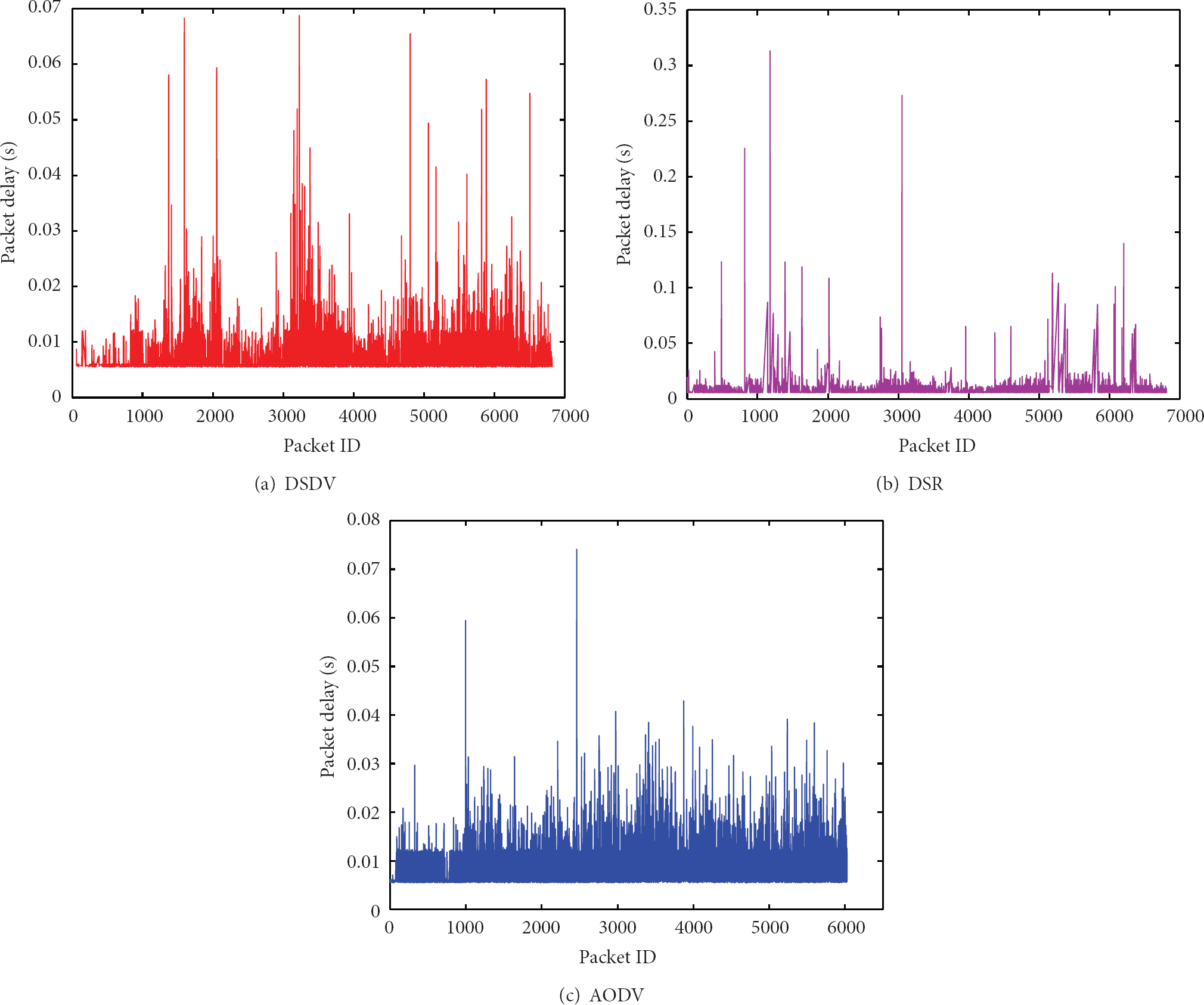
Packet delay of three routing protocols.

(3) Packet Jitter. Figure 5 shows the jitter of data packets using three different routing protocols. The statistical values of them are $(2.356\pm 4.199)$  ms (DSDV, $\alpha =\mathrm{0.95}$ ), $(3.254\pm 10.630)$  ms (DSR, $\alpha =\mathrm{0.95}$ ), and $(4.498\pm 4.498)$  ms (AODV, $\alpha =\mathrm{0.95}$ ), respectively. DSDV shows the most superiority than others. The average jitter of AODV is the biggest among the three protocols. Moreover, the standard deviation of jitter in AODV is larger than that in DSDV. Although the average jitter of DSR is not the largest among the three protocols, DSR has the largest jitter fluctuation among them. This means violent variation exists in the delay of a few data packets sent in DSR. The rapid change of jitter is attributed to the frequent change of network topology and the mechanism of inherent routing update.

Figure 5

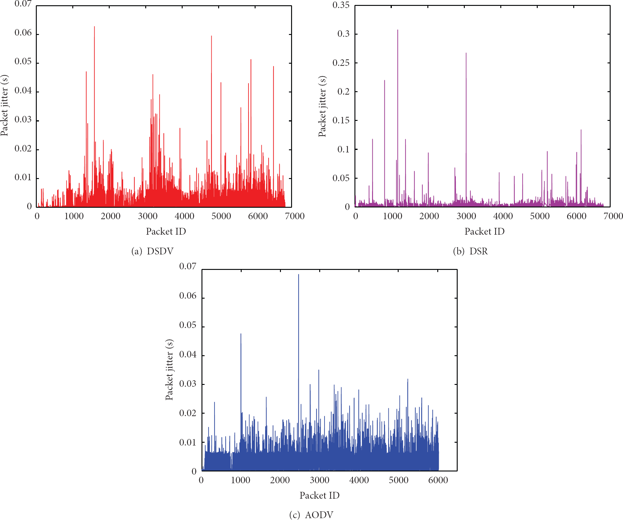
Packet jitter of three routing protocols.

(4) Throughput. Figure 6 shows the throughput comparison of DSDV, DSR, and AODV. All throughputs are ever-increasing with the time in general. This can be attributed to more active nodes to join network communication with time extension. The graph also reveals that AODV has higher throughput than DSR. In DSR, a route is chosen based on the short delay at the instance of route establishment. Although this path may be the best route at that instant, it may be also a route that lacks routing stability or has unacceptably high load. In contrast, AODV has a more robust update mechanism to avoid bottleneck and congestion and eventually improve throughput. In DSDV, high packet loss rate causes throughput to drop.

Figure 6

Throughput comparison of three routing protocols.

(5) Protocol Overhead. Table 3 shows the overhead comparison of DSDV, AODV, and DSR. AODV has the highest overhead among three routing protocols due to three main reasons. Firstly, AODV allows broadcast. Although the discovery packets are broadcasted only when necessary, such as establishing a new route, link breakage, or route error, the broadcast instances will often appear for a fast mobile VANET. Secondly, AODV allows mobile nodes to respond to link breakages and changes in network topology in a timely manner. Thus, numerous routing messages are used to maintain an active route in AODV. Thirdly, AODV is derived from DSDV. It still has similar features of proactive routing protocols. When the network topology is often changed because of the fast mobility of nodes, proactive protocols must send more messages to maintain a valid routing table. The experimental results are shown in Table 3. DSR has the best protocol overhead performance among the three protocols. The DSR protocol is composed of the two main mechanisms of “route discovery” and “route maintenance,” which work together to allow nodes to discover and maintain routes to arbitrary destinations in the ad hoc network. Some measures reducing overhead are adopted in the process of “Route Discovery” and “Route Maintenance” of DSR [21].

Table 3

Overhead of three routing protocols.

Type	DSDV	AODV	DSR
Number of received data packets	5579	5999	5993
Number of sent message packets	25607	39488	1615
Protocol overhead	4.59	6.58	0.27

3.4. Conclusion

Based on the simulation results, we discovered that DSDV achieves marginal better packet delay and packet jitter than AODV and DSR. However, it has significantly higher packet loss rate and the smallest throughout among them. Although DSR has the best protocol overhead performance among three routing protocols, it has poorer jitter and throughput than AODV. As a whole, AODV is more appropriate for the freeway VANET according to the quality of service and the real time of packet delivery. The inherent reason producing this result is the effect of node mobility on the performance of the routing protocol.

4. GPS Based AODV Protocol for V2V Communication [22]

As we can find through the previous protocol evaluation, AODV is appropriate for the dynamic structure with mobile vehicles. The source node will find a route to destination for data transmission. To find a route to the destination, the source broadcasts a route request packet (RREQ). The node receiving RREQ will reply a route reply packet (RREP) to the reverse path that RREQ went through if it is the destination of RREQ or if it has a recent route to the destination. Otherwise, the node will broadcast RREQ until either of the two situations above occurs. As RREP traverses back to the source, the nodes along the path enter the forward route into their routing tables. If a node leaves the network, the node that discovers this broken link will send a link failure notification (RERR) to the precursors. The RERR goes upstream until it reaches the source. The source will thereafter restart route discovery process if needed [23].

However, AODV is dedicated for MANET, and modification is necessary for VANET applications [24]. Since nodes in VANET are fast moving vehicles, the topology of the network changes all the time, making the position and velocity of the node critical factors while finding the routes. Therefore, besides conventional topology-based routing protocol (such as AODV), position-based routing protocol, which primarily uses the position information obtained by GPS to find a route, is applied in VANET [25].

In recent years, many researchers have tried to combine two types of routing together. In [26], Kim et al. proposed AODV-RRS which restricts the number of forwarding RREQs according to the concepts of stable zone and caution zone. PAODV [27] restricts the number of flooding RREQs based on the distance between current node and its neighbors. Both of them have similar mechanism and reduce the number of broken links. DAODV [28] establishes a route depending on the direction and position of source, intermediate, and destination node. Although it also reduces the number of broken links, DAODV assumes that source node knows the direction and position of all the nodes in the network. Actually this is impossible with the current GPS devices. We should find some mechanisms to get the geographic information of all the nodes. Thereby, in [29], Asenov and Hnatyshin proposed GeoAODV routing protocol. Each node will maintain an additional table, geotable, to keep track of the geographic information of all the nodes. RREQs are restricted flooding in the region determined by the geotable. However, it costs more resources to maintain two tables.

We go a step further in this section by proposing a GPS based AODV (GBAODV), which enhances the overall performance of AODV in VANET. In order to be attainable in physical implementation, GBAODV assumes that each node only knows its own position and velocity. Without maintaining a geotable [29], GBAODV is much more concise than GeoAODV.

4.1. Overview of GBAODV

With current GPS device, we can obtain the longitude (x coordinate) and latitude (y coordinate) of current node, and calculate the speed in each direction with two successive sets of coordinates. Without maintaining a geotable, we add geographic information into routing table to make the algorithm concise.

There are two main features in GBAODV. First is to reduce the number of RREQs. The node receiving an RREQ packet will check the distance and motion trend between the precursor and itself, so as to decide if this RREQ should be broadcasted. By restricting these flooding RREQs, it will avoid lots of packet collisions in the network. As a result, the packet delivery ratio and throughput of the network can be raised. Second is to mark the route according to the positions and velocities of source, intermediate, and destination. Higher mark means higher stability. Consequently, every node will choose a route with higher mark.

These two features require specifying flooding rules and marking standards, as well as some modifications in the routing table and routing packets.

4.2. Modified Structure of Routing Table, RREQ, and RREP

(1) Modified Routing Table. Original routing table contains the IP addresses of next hop and destination, sequence number of destination, and total hops. The routing table will update if the sequence number of destination is larger or total hops is less. We added the position and velocity of the destination node and the mark of this route into the routing table. Besides the two conditions above, the routing table will update when the mark is larger, which means that the route path is more stable.

(2) Modified Frame Structure of RREQ. We inserted position (x, y coordinates) and velocity (x, y direction) of the source and current node into RREQ packet. We also applied a reserved segment to record the mark of the route link from source to precursor.

(3) Modified Frame Structure of RREP. RREP is modified similar to RREQ. We inserted position and velocity of the destination and current node into RREP packet. We also applied a reserved segment to record the mark of the route from destination to current node.

4.3. Flooding Rules and Marking Standards

(1) Flooding Rules. Let d stand for the distance between the precursor and current node and R stand for the maximum transmission distance of the wireless card. The flooding rules are as follows.

If $(d<\mathrm{0.4}\hspace{0.17em}R\parallel (d>\mathrm{0.8}R\&\&d\hspace{0.17em}\hspace{0.17em}\text{is}\hspace{0.17em}\hspace{0.17em}\text{increasing}))$

•  

discard RREQ;

Else,

•  

broadcast RREQ.

The coefficients 0.4 and 0.8 are chosen empirically. We conducted simulations with the combinations of these coefficients to study numbers of RREQs and RERRs, packet loss ratio, and average end-to-end delay. Results show that the combination of 0.4 and 0.8 is the best among all.

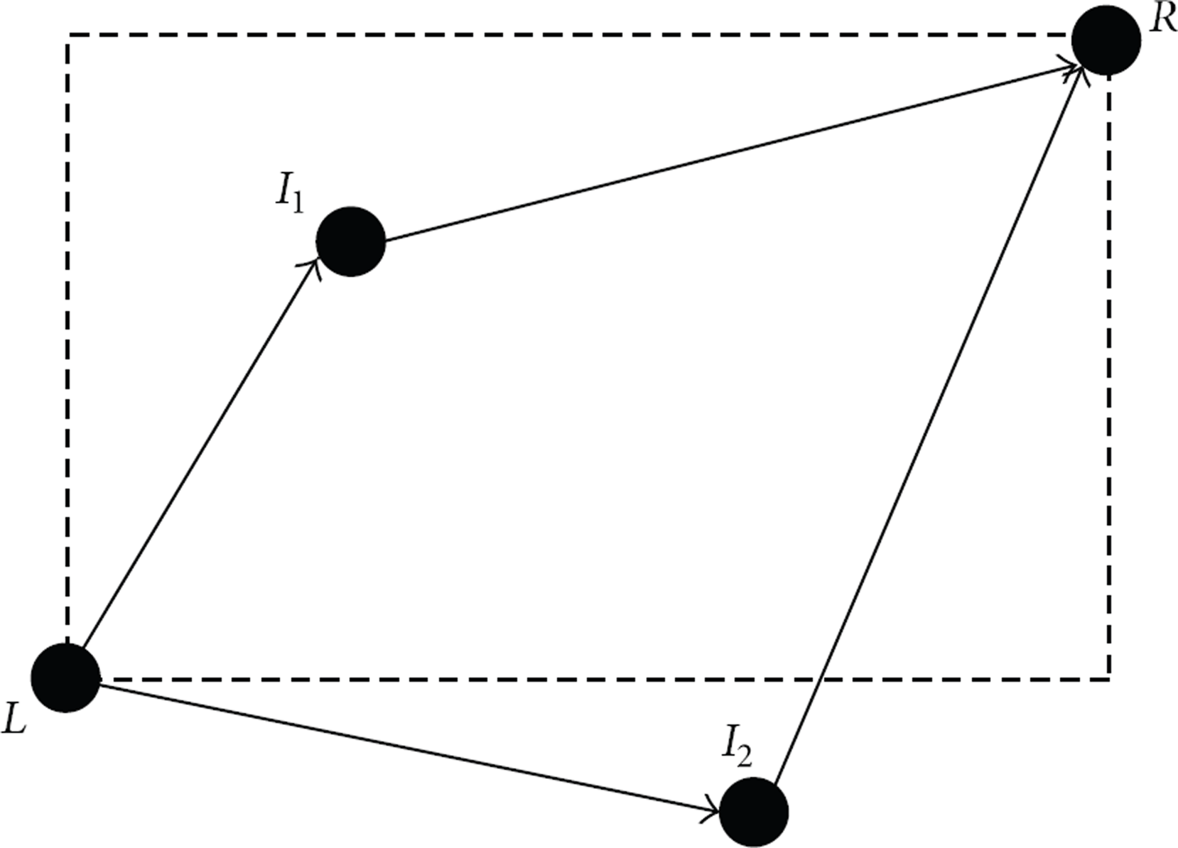
In Figure 7, B, C, and D will broadcast the RREQ received from P, while A and E will discard it.

Figure 7

B, C, and D will broadcast RREQ received from P.

(2) Marking Standards. As illustrated in Figure 8, let $L{D}_c$ stand for the current distance between node L and node I, $L{D}_l$ stand for this distance a moment later, $R{D}_c$ stand for the current distance between node I and node R, and $R{D}_l$ stand for this distance a moment later. We specify the marking standards as follows:

$$\begin{array}{cc}& \text{mark}=\mathrm{2}\mathrm{sgn}\left(L{D}_c-L{D}_l\right)+\mathrm{2}\mathrm{sgn}\left(R{D}_c-R{D}_l\right)+C,\end{array}$$

(2)

where $\mathrm{sgn}()$ is a signum function.

Figure 8

Different mark for different regions.

C is a constant:

$$\begin{array}{cc}& C=\{\begin{array}{cc}0\hfill & \text{if}\hspace{0.17em}\hspace{0.17em}I\hspace{0.17em}\hspace{0.17em}\text{is}\hspace{0.17em}\hspace{0.17em}\text{in}\hspace{0.17em}\hspace{0.17em}\text{the}\hspace{0.17em}\hspace{0.17em}\text{dashed}\hspace{0.17em}\hspace{0.17em}\text{rectangle}\hfill \\ -3\hfill & \text{if}\hspace{0.17em}\hspace{0.17em}I\hspace{0.17em}\hspace{0.17em}\text{is}\hspace{0.17em}\hspace{0.17em}\text{out}\hspace{0.17em}\hspace{0.17em}\text{of}\hspace{0.17em}\hspace{0.17em}\text{this}\hspace{0.17em}\hspace{0.17em}\text{rectangle}.\hfill \end{array}\end{array}$$

(3)

−3 is chosen experimentally according to simulations.

Since the transmission distance of wireless LAN card is limited, geographic distance of each hop is the key factor that affects the quality of communication. If the distance stays unchanged, then the route is really stable so that the source and destination can communicate steadily. If the distance is increasing, it is possible that one node in this route will exceed the transmission distance soon. If the distance is decreasing, then after some time, the two nodes may cross over and start to depart. It is better than increasing distance, but not as good as unchanged distance. So we set two values for each changed distance: 0 for each decreasing distance and −2 for each increasing distance, as shown in (2).

To find a path to the destination, the source broadcasts an RREQ containing the position and velocity of source and preset a standard mark value.

As illustrated in Figure 9, when a node receives an RREQ the following will occur.

• (i)

If it does not have a route to the source node, it will insert the route RREQ into its routing table.

(ii)

If it has a route in routing table but the route needs to be updated, it will update routing table.

(iii)

If it is the destination or has a route to destination, it will create an RREP in which the mark is a standard value (if it is the destination) or is obtained from routing table (if it has a route to destination).

(iv)

If it is a node besides (3) and satisfies the broadcasting conditions (refer to flooding rules), it will add the mark of source→precursor→current to the present mark in RREQ. It will also update the position and velocity of current node in RREQ.

Figure 9

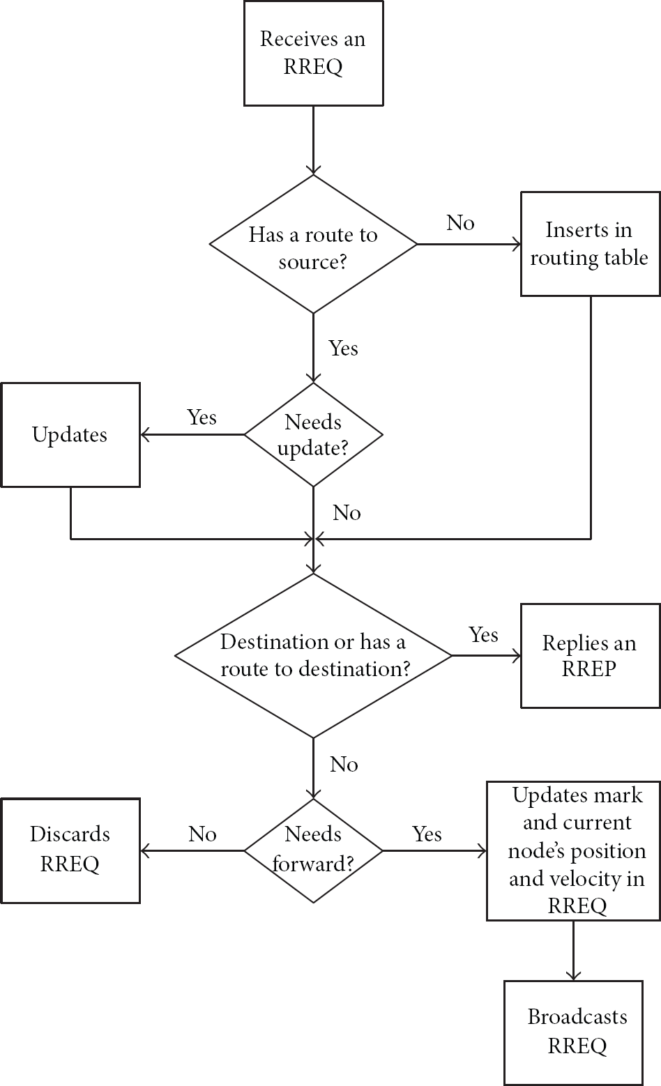
Flowchart of processing RREQ.

As illustrated in Figure 10, when a node receives an RREP the following will occur.

• (i)

If it does not have a route to the destination, it will insert the route, which RREP goes through, into its routing table.

(ii)

If it has a route in routing table but the route needs to be updated, it will update routing table.

(iii)

If it is the destination of RREP (i.e., the source of RREQ), it will insert the route into routing table.

(iv)

If it is a forwarding node, before unicasting RREQ, it will add the mark of source→precursor→current to the present mark in RREP. It will also update the position and velocity of current node in RREQ.

Figure 10

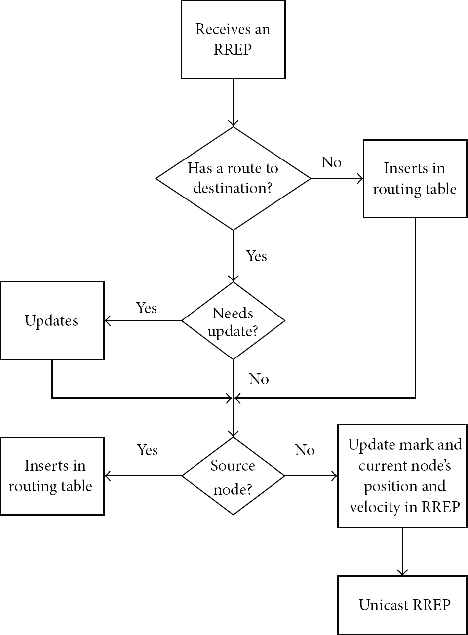
Flowchart of processing RREP.

4.4. Simulation Setup

(1) Simulation Tools. We chose VanetMobiSim 1.1 [30] for traffic simulation. This software can generate a traffic flow in the format suitable for NS2 [31], which can load GBAODV for network simulation.

With VanetMobiSim, we import maps from the US Census Bureau TIGER/Line database [32], which includes complete coverage of the United States, Puerto Rico, and so forth. Moreover, VanetMobiSim supports for multilane roads, differentiated speed constraints, and traffic light signals at intersections. All the vehicles can be set to Intelligent Driver Model with Lane Changing (IDM_LC) [33, 34]. For these reasons, the scenario in traffic layer is quite authentic, which makes the simulation in network layer reliable.

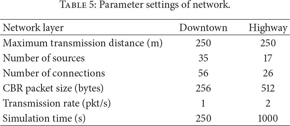
(2) Parameter Settings. In our simulation, we observed two types of traffic models: downtown and highway. TGR11001 [32] (district of Columbia, WA) is chosen as downtown map and TGR36001 [32] (Albany county, NY) is chosen as highway map. Multilanes and traffic lights are involved. All the vehicles follow the IDM_LC driving model. Tables 4 and 5 are the parameter settings of traffic and network simulation. Traffic flow and CBR (constant bitrate) data flow are both generated randomly.

Table 4

Parameter settings of traffic.

Traffic layer	Downtown	Highway
Area (m2)	$\mathrm{1000}\times \mathrm{1000}$	$\mathrm{1000}\times \mathrm{1000}$
Number of lanes	3	3
Maximum number of traffic lights	10	None
Speed (km/h)	20~80	60~120
Simulation time (s)	250	1000

Table 5

Parameter settings of network.

Network layer	Downtown	Highway
Maximum transmission distance (m)	250	250
Number of sources	35	17
Number of connections	56	26
CBR packet size (bytes)	256	512
Transmission rate (pkt/s)	1	2
Simulation time (s)	250	1000

4.5. Simulation Results

(1) Downtown Model. Figure 11 illustrates that the number of RREQs received per node per second is reduced by about 50%. This is caused by the application of flooding rules. In addition, we can notice that although it is normalized by the number of nodes, the number of RREQs still increases with the number of nodes. This means larger number of nodes induces larger amount of RREQs broadcasted in the whole network. Therefore, it is significant to reduce the broadcasted RREQs especially in high density traffic.

Figure 11

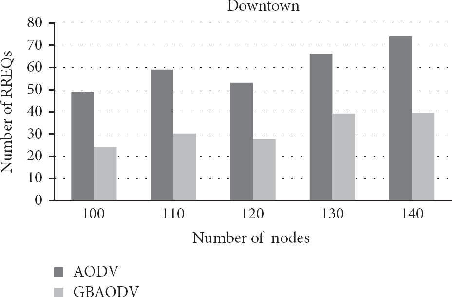
Number of RREQs received downtown per node per second.

Figure 12 illustrates the number of RERRs sent per connection. The number of RERRs is also reduced a lot which means broken links have decreased a lot. This is an attribute to the application of marking standards since we choose every connection with high stability.

Figure 12

Number of RERRs sent in downtown scenario per connection per second.

Figures 13 and 14 illustrate the packet loss ratio and average end-to-end delay. Compared with Figures 11 and 12, they show that packet loss ratio and average end-to-end delay are positive correlated to the numbers of RREQs and RERRs, because reducing the number of RREQs contributes to avoiding large amount of packet collisions in the network. Meanwhile, reducing the number of RERRs (i.e., broken links) could smooth communication.

Figure 13

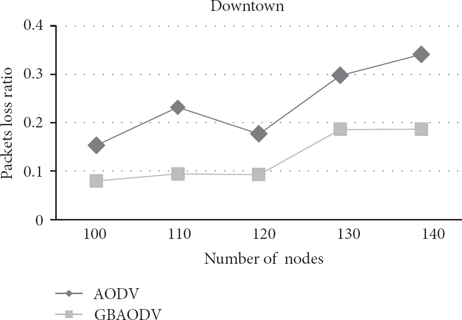
Packet loss ratio in downtown scenario.

Figure 14

Average end-to-end delay in downtown scenario.

(2) Highway Model. The number of RREQs received per node per second is reduced by more than 50% (illustrated in Figure 15). Figure 16 shows that the number of RERRs sent per connection is also reduced. We also note that with the increase of number of nodes, the reduction of RERRs (i.e., broken links) increases. This means GBAODV is more efficient in high density traffic scenario. The conclusion is verified by Figure 17 (packet loss ratio) and Figure 18 (average end-to-end delay). Compared with Figures 13 and 14, the improvement of network performance is not as sharp as that which we obtained in downtown model.

Figure 15

Number of RREQs sent in highway scenario per node per second.

Figure 16

Number of RERRs sent in highway scenario per connection per second.

Figure 17

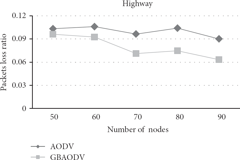
Packet loss ratio in highway scenario.

Figure 18

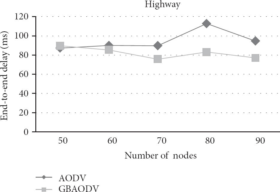
Average end-to-end delay in highway scenario.

The main reason is that the node density in highway model is relatively low. Firstly, lower node density leads to less number of RREQs flooding in the network (referring to Figures 11 and 15). The number of RREQs received per node per second in highway model is about 80% of that in downtown model. Therefore, packet collision in highway is slighter than in downtown. Although GBAODV weakens packet collision, it achieves no big improvement. Secondly, lower node density provides fewer choices of stable routes. If we restrict the number of RREQs, the effect caused by skipping some stable routes is larger than that in downtown model. That is the reason why the reduction of the number of RERRs in highway model is less than that in downtown model (referring to Figures 12 and 16).

To conclude, GBAODV is much better than AODV in both models. It releases the load of the network (less number of RREQs), reduces broken links and packet loss ratio, and shortens average end-to-end delay.

5. Vehicle Information Sinking Network Based on Mobile Nodes [35]

Aside of the mobile V2V network, the information from the vehicles should also be sent to the sink node, which will be normally performed by the roadside infrastructure. However, the construction of these infrastructure networks is expensive in both funding and time. Hence, mobile node acted by vehicles can firstly serve as the sinking port. This section elaborates a data gathering algorithm based on swarm intelligence. Although the computational resource and energy source of the on-board computer in vehicles, compared to field wireless sensor nodes, is abundant, applications may need to be extended to bicycle riders, with limited energy source. The transmitted information in the future will be extended as there will be applications aside of accident reporting, such as cloud computation, media access, and entertainment through the V2V and V2I network. Hence, in order to maximize the overall network efficiency, communication load of each vehicle node ought to be balanced.

Much reference can be made from the current research on hand-held devices such as 3G mobile phone and PDA, which play role as mobile sink of wireless sensor network (WSN) node in applications [36, 37]. Thus the algorithm for the data gathering application should support the sink node mobility. It is a challenge in WSN algorithm design.

Based on the application of the sensor network, the data delivery model to the sink node can be categorized into three types: query-driven, event-driven, and continuous. In query-driven model, the sink node generates a query, and then a temporary route is built. The node which is checked receives query and returns result, for instance, DD [38] and ACQUIRE [39]. In event-driven model, because the event rate is much lower without temporal and spacial information, the event node triggers the data transmission and temporary route building, such as Rumor routing [40] and TTDD [41]. Focusing on these two types of data transmission model, the routes are temporary, so the sink node mobility has little influence on data transmission. In the continuous delivery model, each sensor collects data periodically and sends data to the sink node for gathering. In data gathering application, the sink node builds the route usually; for instance, it has been concluded in TEEN [42], APTEEN [43], and MINA [44]. However, movement of the sink node often results in broken links. If the route is rebuilt frequently, not only the network energy consumption will be large, but also the regular data transmission will be blocked by the network storm, which will result in massive broadcasting messages.

Sink mobility brings new challenges in data gathering application, although some protocols and mechanisms have been proposed in recent years, such as TDD, SEAD [45], CODE [46], and others in [47, 48]. TTDD uses a grid structure so that only sensor located at the grid points needs to acquire the forwarding information. The route path for the moving sink node is maintained and refreshed by agent nodes. When there are several data sources in the network, the overhead is large. Meanwhile, the route needs to be rebuilt when the sink node moves out of the grid. SEAD protocol designs a dormancy mechanism for the nodes in grid to reduce energy consumption. The current route extends and recovers by itself while the sink node moves, but time delay remains a problem. CODE does not need to rebuild global path, but it needs other routing protocols to support, so the protocol is more complex. A local routing restoring mechanism is proposed in [47] that the sink node sends Sink_Claim message periodically. This message is used for the sink node detection. The sensor node would change its status according to this message. The main problem of this method is the large consumption caused in sending the Sink_Claim message in high frequency. Meanwhile, the throughput becomes smaller. As described in above, TTDD, SEAD, CODE, and others in [47, 48], they are all designed for query-driven or event-driven transmission model, so these methods are not much suitable for data gathering application.

For data gathering application in V2I, this section studies the equilibrium mechanism and proposes a swam intelligence data gathering algorithm for mobile sink (SIDGMS). The idea of SIDGMS algorithm is derived from swarm intelligence such as ants. In this algorithm, each vehicle node is a smart individual but with limited knowledge. SIDGMS defines two simple rules to describe the data forwarding. The problem how to choose next hop becomes multiobjective programming, which considers both the delay and load of the network. To solve link-break problem, a method of the power control for the Sink beacon message is proposed.

5.1. SIDGMS Algorithm

The idea of SIDGMS algorithm is derived from swarm intelligence. The preying behavior, as a typical behavior of swarm intelligence, has simple rules. If an individual discovers food, others will observe and study local behavior from the individuals in the region. As a result, everyone in group can find food.

Each node in a wireless sensor network (WSN) system has limited computational ability, memory space, energy, and wireless transmission range, so the nodes can only exchange information with neighbor nodes within the wireless communication range.

Sink node can be regarded as food source, and the process of data gathering can be regarded as swarm foraging action. The sink node and other nodes are mapped on Figure 19.

Figure 19

The structural relationship between the sink and vehicles.

The principle of data gathering works as below.

• (i)

The sink node broadcasts beacon periodically, which contains its current location information.

(ii)

The internal nodes discover the sink node directly and start the data transmission with the sink node.

(iii)

Meanwhile, the external nodes detect the data transmission between the internal nodes and the sink node, which helps the external nodes discover the sink indirectly and triggers the data transmission between them if needed.

(1) SIDGMS Algorithm Mechanism. In this algorithm, the nodes in WSN system can be separated into two types, the sink node with mobility and the sensor nodes. Two messages are defined as below.

Message  1. SINK_BEACON (sinkInfo), which is sent by the sink node to inform sensor nodes. sinkInfo includes the location component ( $x,y$ ) and sequence number seq, which is incremental.

Message  2. SENSOR_DATA (nextAddr, data, sinkInfo, loadInfo), which is sent by sensor node. The sensor node collects its vehicular information (data) and then forwards it to next-hop node (nextAddr). The latest sink location component (sinkInfo) and load information component (loadInfo) are included in this message.

During the data transmission period, the sensor node saves location component of the sink node and refreshes this component once it receives a new one, which could be identified by the sequence number component (seq). At the same time, the sensor node changes its status according to the SINK_BEACON message. The status of sensor node is defined as follows

Definition 1.

If sensor node receives the SINK_BEACON message at a interval time T (T is the periodic time of SINK_BEACON), the sensor node marks its status as Sink Adjacent (SA). Otherwise, it marks its status as Nonsink Adjacent (NSA).

According to different status of the sensor node, the algorithm has different data forwarding rules, which are listed as follows.

Rule  1. If the sensor node status is SA, the data is forwarded to the sink node directly.

Rule  2. For any sensor node in NSA status, it has two criteria to choose next hop. The first criterion is for less delay, and the other is for load balance of the network.

Generally, the sensor node which is closer to the sink node has less jumping hops, so its delay is smaller.

For any sensor node i, the distance from the sink node is calculated according to (4) as below:

$$\begin{array}{cc}& d\left(i\right)=\sqrt{{\left(x_i-x_{\text{sink}}\right)}^{\mathrm{2}}+{\left(y_i-y_{\text{sink}}\right)}^{\mathrm{2}}}.\end{array}$$

(4)

For any sensor node i which is in NSA status, the best sensor node for next hop considering the fast transmission is solved according to (5):

$$\begin{array}{cc}& J=\arg \underset{j\in N\left(i\right)}{\min }d\left(j\right),\end{array}$$

(5)

where $N(i)$ denotes the neighbor nodes of the node i.

It is a complicated problem to calculate the loading of each sensor node. However, it can be estimated in two ways. In one hand, the key to maximize the WSN lifetime is to reduce energy consumption in each sensor node. We assume that each sensor node has the same hardware equipment. Thus the remaining battery energy in each node should be considered.

On the other hand, the time to forward messages in a WSN system is closely related to the network performance, such as the packet loss rate, time delay, and network congestion. Therefore, the total time of forwarding action could be used as indicator of the network loading. It could be denoted by the number of package buffer queue.

This mathematical model is elaborated as below.

Definition 2.

The loading of sensor node in WSN system is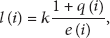

$$\begin{array}{cc}& l\left(i\right)=k\frac{\mathrm{1}+q\left(i\right)}{e\left(i\right)},\end{array}$$

(6)

where $l(i)$ denotes the loading of the sensor node i, $e(i)$ is the battery dump energy, $q(i)$ is the mean number of the packages in the buffer queue, and k is scale factor.

For any sensor node i which is in NSA status, the best sensor node for next hop considering the load balance is calculated by

$$\begin{array}{cc}& J=\arg \underset{j\in N\left(i\right)}{\min }l\left(j\right).\end{array}$$

(7)

Definition 3.

For the criterions of Rule  2, ${\lambda }_d$ is defined as the distance weight coefficient with the sink node, and ${\lambda }_l$ is defined as the loading weight coefficient for the sensor node. ${\lambda }_d\ge \mathrm{0}$ , ${\lambda }_l\ge \mathrm{0}$ , and ${\lambda }_d+{\lambda }_l=\mathrm{1}$ .

The final optimization considers both the aspects of faster transmission and power balance, as below:

$$\begin{array}{l}\underset{j\in N\left(i\right)}{\min }\hspace{1em}({\lambda }_d\left|d\left(j\right)-d^{\mathrm{0}}\right|+{\lambda }_l\left|l\left(j\right)-l^{\mathrm{0}}\right|)\\ \text{s}.\text{t}.\phantom{.\mathrm{0}.}d\left(j\right)<d\left(i\right),\hspace{1em}{\lambda }_d\ge \mathrm{0},\\ \phantom{00.0000}{\lambda }_l\ge \mathrm{0},\hspace{1em}{\lambda }_d+{\lambda }_l=\mathrm{1},\end{array}$$

(8)

where $d^{\mathrm{0}}$ is the minimum distance and $l^{\mathrm{0}}$ is minimum loading. The distance weight coefficient ${\lambda }_d$ and the loading weight coefficient ${\lambda }_l$ are interrelated with application. For some applications which require high real-time response, ${\lambda }_d$ would be increased. For some applications which focus on the energy equilibrium, ${\lambda }_l$ will be increased. $d(j)<d(i)$ to prevent looping back.

5.2. Power Control Strategy

(1) Node Coverage Radius. The sink node broadcasts SINK_BEACON periodically. However, no matter how frequently the sink node broadcasts the SINK_BEACON message, packet loss would happen. That is because the linkage between the sink node and a sensor node in boundary area is fragile, due to the movement of the sink node. This case is shown in Figure 20, in which all the sensor nodes and sink node have the same transmission radii.

Figure 20

Same covering radius.

In order to solve this problem, we propose a new strategy to avoid link breaking, as shown in Figure 21. The transmission radius of the sink node is smaller than that of the sensor nodes. At present, most of the microcontrollers for WSN can support this by power control, such as CC2430, CC1100, and MC132x.

Figure 21

Different covering radius.

How to determine the transmission radius of the SINK_BEACON? As proposed in [49], with assumptions that the density of nodes is uniform and all nodes in WSN domain are subject to the Poisson distribution, the probability that m nodes exist in area S is

$$\begin{array}{cc}& P\left(X=m\right)=\frac{{\left(\rho S\right)}^m{\dot{e}}^{-\rho S}}{m!}.\end{array}$$

(9)

Therefore, the problem of radius r could be translated into (10) as follows:

$$\begin{array}{cc}& P\left(X>\mathrm{0}\right)=\mathrm{1}-P\left(X=\mathrm{0}\right)\ge \alpha ,\end{array}$$

(10)

where α is the confidence, which denotes the probability that SA node appears.

Finally, the radius r can be determined as

$$\begin{array}{cc}& r\ge \sqrt{\frac{\ln \left(\mathrm{1}-\alpha \right)}{\pi \rho }}.\end{array}$$

(11)

(2) Cycle Time of SINK_BEACON. It is shown in Figure 22. In this case, we assume the movement velocity of the sink node is V, the transmission radius of SENSOR_DATA message is R, and the transmission radius of SINK_BEACON message is $r\mathrm{\hspace{0.17em}\hspace{0.17em}}(r<R)$ . Hence, cycle time of the SINK_BEACON message should satisfy this condition: $VT\le R-r$ .

Figure 22

Partial address routing.

Therefore, the cycle time of the SINK_BEACON is calculated as follows:

$$\begin{array}{cc}& T\le \frac{R-r}{V}.\end{array}$$

(12)

For example, if the transmission radius of SENSOR_DATA is 100 m, the transmission radius of SINK_BEACON is 50 m, and the moving velocity of the Sink node is 10 m/s, representing that the sinking vehicle moves slowly on the road; the max cycle time of SINK_BEACON is 5 s.

5.3. Experiment and Analysis

The simulation for evaluating SIDG-MS algorithm is implemented with NS2.

(1) Implementation of SIDG-MS Algorithm. The sink node takes charge of sending SINK_BEACON and data gathering. The pseudocode is listed in Pseudocode 1.

Pseudocode 1: The sink node pseudocode of SIDG-MS.

timerStart(T, PERIOD_TYPE)

while (haveEnergy)

  if (timerFired)

   sendMsg(SINK_BEACON, sinkInfo)

  else if (receivedMsg)

   renderMsg()

  end

end

The sensor node collects vehicular data and forwards to the sink. It runs in distributed mode and the pseudocode in every node listed in Pseudocode 2.

Pseudocode 2: The sensor node pseudocode of SIDGMS.

status:= NSA

while (haveEnergy)

   switch (receivedMsg)

   case: SINK_BEACON

    status:= SA

    recordSinkInfo()

    timerStart(T, SINGLE_TYPE)

    break

   case: SENSOR_DATA

    if (toSelf)

      computeNextHop()

      forward()

    else

      recordInfo()

    end

    break

  end

  if (timerFired)

  status:= NSA

  end

  if (sensorDataReady)

  computeNextHop()

  sendData()

  end

end

(2) Test Scenario. The simulation scenario is designed according to a plane area, which is 800 meters wide and 800 meters long. There are totally 401 nodes in this WSN system, including 1 sink node and 400 sensor nodes. The sink node moves randomly in the network with a constant speed 10 m/s. The sensor node collects the sensor data at a time interval every 10 s and its initialization energy is 50 J. Other simulation parameters are listed in Table 6.

Table 6

Simulation parameters.

Parameter	Value
Scene size	$\mathrm{800}\times \mathrm{800}$ (m)
Node number	400 node + 1 sink
Mac	802.11
Application	CBR
Packet size	1024
Queue length	10
Channel model	Two-ray ground

We assume the energy consumption for collecting data is $\mathrm{1}\times \mathrm{1}{\mathrm{0}}^{-\mathrm{5}}\hspace{0.17em}\text{J}$ , the energy consumption for receiving data is $\mathrm{5}\times \mathrm{1}{\mathrm{0}}^{-\mathrm{5}}\hspace{0.17em}\text{J}$ , and the energy consumption for transmitting data is $\mathrm{1}\times \mathrm{1}{\mathrm{0}}^{-\mathrm{4}}\hspace{0.17em}\text{J}$ . The value of SINK_BEACON transmitting radius calculated according to (11) is larger than 50 meters $(r\ge \mathrm{50}\hspace{0.17em}\text{m})$ ; in this simulation r it is initialized as 80 meter. The transmission radius of the sensor node for SENSOR_DATA message is initialized as 150 m. The periodic time of SINK_BEACON calculated according to (12) is smaller than $\mathrm{7}\hspace{0.17em}\text{s}\mathrm{\hspace{0.17em}\hspace{0.17em}}(T\le \mathrm{7}\hspace{0.17em}\text{s})$ , so T is initialized as 5 seconds.

(3) Simulation Result and Analysis. The more incoming and outgoing message in MAC layer, the larger energy consumption will be. Therefore, we calculate the network energy consumption of every interval by counting the communication message in MAC layer is. The simulation result is shown in Figure 24, which illustrates the energy consumption character of SIDGMS, Huang et al. [47], and Lee et al. [48] algorithms. When the sink node is in motion, the energy consumption in literature [47] increases because the route path increases. In the algorithm of literature [48], the route path to the sink node is checked during each message packet transmission, so the energy consumption runs at a constantly high level. In SIDGMS algorithm, the location of the sink node could be refreshed during the motion. Thus this strategy has less energy consumption.

The network lifetime is defined as the time period until one of the nodes dies. The simulation result with different methods is shown in Figure 23. The lifetime in literature [48] is the shortest due to the large energy consumption, such as many refreshing actions for route path. The lifetime in literature [47] is shorter than SIDGMS algorithm because there is no optimization for load balance. Some node's loadings are too heavy to support long lifetime.

Figure 23

Network lifetime comparison.

Figure 24

The energy consumption comparison between three methods.

Time delay is an important factor of WSN system, we analyze it by monitoring the CBR stream. The simulation result is shown in Figure 25. Time delay with the SIDGMS algorithm is significantly lower than the other two algorithms.

Figure 25

Time delay comparison.

6. System Integration and Experiments [7]

To test the communication system, we developed a series of hardware as experimental platforms.

6.1. Platform Integration Architecture

Figure 26 shows the system architecture including two major components: onboard integration subsystem and V2V portable subsystem.

Figure 26

Platform integration architecture.

6.2. Integration for Onboard Subsystem

Onboard subsystem is full version for collision detection and classification, so all sensors as shown in Table 1 are installed onboard. Some main sensors are shown in Figure 27.

Figure 27

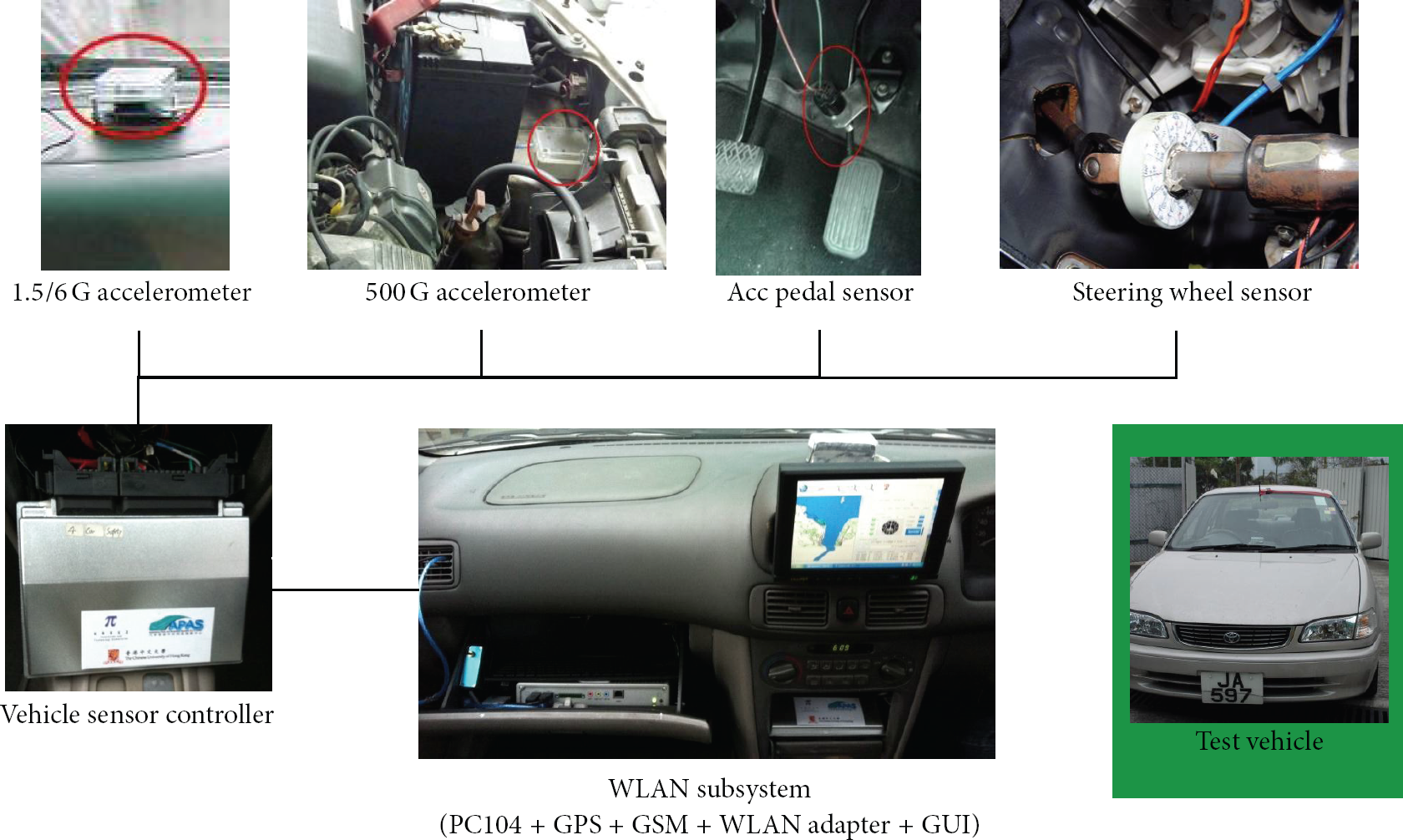
Onboard integration subsystem.

6.3. Integration for V2V Portable Subsystem

In order to design low cost platform for V2V application, we also need to develop a portable system to be installed on others test car. A series of portable V2V nodes have been developed and used for real road test, as shown in Figure 28.

Figure 28

V2V portable subsystem.

Currently, we implement GBAODV based on AODV-UU [50]. Two threads are running under one main process. One is for routing in the network and the other is for reading GPS data through serial port directly.

Environment and devices for network test include

• (i)

Linux Fedora 7,

(ii)

PC104 consortium [51],

(iii)

Ralink RT2500 series wireless LAN card,

(iv)

SiRF StarIII GPS module,

(v)

touch screen and keyboard.

6.4. Road Test Scene

In this section, different experiments are conducted to demonstrate the functions and performance of the integrated system. In these experiments, the key vehicle is a Toyota Corolla, equipped with the full version system, including WLAN-based component, GPS component, GPRS component, hazardous driving behavior detection subsystem, and collision detection and analysis subsystem. Aside of that, we prepared eight sets of portable systems. These portable systems include WLAN-based component and GPS component. The scene of experiments is the road near Hong Kong Science Park and the corresponding driving path is marked as a blue path in Figure 29.

Figure 29

The scene of experiments: Science Park, Hong Kong.

6.5. V2V Communication Test

In this experiment (Figures 30 and 31), all vehicles are driven along a line with 30 km/hr. Different alarm signals are triggered manually by each of the vehicles randomly. The source sends 100 PING messages to destination continuously. The V2V communication system is then evaluated by checking whether the other vehicles can receive the PING message caused by status changing. The test result is shown in Table 7.

Table 7

Average packet loss ratio.

Number of nodes	AODV	GBAODV
4	45.5%	61.7%
5	63%	59%
6	73%	59%
7	56%	54.3%
8	51.5%	41%

Figure 30

Vehicle experiment.

Figure 31

GUI for vehicle experiment.

GBAODV performs better than AODV in general. Although the packet loss ratio is large, this is acceptable. Since there are barriers, such as buildings, in the experiment environment, the signal attenuates rapidly. The packet loss ratio after one hop is approximately 20%. PING is round trip message. If source and destination cannot communicate directly, PING message traverses at least 4 hops. Therefore, the packet loss ratio is at least

$$\begin{array}{cc}& \mathrm{1}-{\left(\mathrm{1}-\mathrm{0.2}\right)}^{\mathrm{4}}=\mathrm{0.5904}.\end{array}$$

(13)

This is close to the experiment results. If the environment is clear enough, the results should be better.

7. Conclusion

In this paper, we presented a vehicle safety enhancement system based on wireless communication. The system can obtain vehicular signals, classify hazardous information, and make decision to trigger different actions to prevent the accident from occurrence or deterioration. To enhance the network performance, we evaluated DSDV, DSR, and AODV protocols and adopted AODV as the benchmark protocol. Thereafter, GPS information is integrated into AODV to further upgrade to GBAODV, which reduces packet loss rate and end-to-end delay, especially for downtown application in VANET. This paper also addresses V2I routing, by proposing the SIDGMS, which balances delay and network load. Simulation validates the V2I algorithm. Finally, we evaluate the V2V system by on-road test.