
Abstract
We focus on the need for traversability analysis of vehicles with convolutional neural networks. Most related approaches to traversability analysis of vehicles suffer from the limitations imposed by extracting explicit features, algorithm scalability, and environment adaptivity. In views of this, an approach based on the convolutional neural network (CNN) is presented to traversability analysis of vehicles, which can extract implicit features. Besides, in order to enhance the training speed and accuracy, preprocessing and normalization are adopted before training. The experimental results demonstrate that our method achieves high accuracy and strong robustness.
1. Introduction
In recent years, there has been a great deal of interests in the field of visual-based traversability analysis of vehicles' travelling directions. It has been regarded as one of the major topics in the area of intelligent transportation.
Research for traversability analysis based on the image understanding can be divided into two parts, one is the methods based on reconstruction and the other is based on recognition [1]. Methods based on reconstruction can judge the traversability from the perspective of space, which is difficult to avoid the serious ambiguity, smaller range of reconstruction, and bad real-time capability of three-dimensional reconstruction [2]. Methods in image understanding based on recognition method, mostly are based on modeling and template matching algorithm, a general neural network, support vector machine (SVM), self-supervised learning, and statistical learning methods. All these methods by themselves are limited in what they must extract explicit characteristics of the target in complex extraction process. In the process, important information may be easy to lose. In addition, these methods also have poor environmental adaptability.
In order to simplify the process of feature extraction and also improve the algorithm scalability and environment adaptivity, a convolutional neural network is proposed in this paper. As noted in [3], convolutional neural networks offer state of the art recognizers for a variety of problems, such as vehicle detection [4], pedestrian tracking [5, 6], obstacle detection [7], face detection [8–10], robot navigation [1, 5], and off-road terrain classification [11]. Generally speaking, the convolutional nets can be used to implicit characteristics extraction, which is specifically designed to deal with the variability of 2D shapes and reduce the algorithm complexity (CNN, LeCun and Bengio, 1995). Also, it can naturally produce invariance to translation, scaling, and some rotation. In addition, the convolutional nets can also reduce the computational complexity and improve the adaptive capacity to environment.
The remainder of this paper is organized as follows. In Section 2, the processing and normalization for original images were done to improve removal of light effects. Also, image labeling is accomplished in this section. Then, the images are normalized in geometry, so that we can acquire suitable training samples for the convolutional nets. Section 3 describes the convolutional neural network which has the advantages of incorporate weights sharing and invariableness to translation and some rotation and Section 4 shows details about the recognition and classification process; experimental results are presented and analyzed in details. Finally we conclude this paper in Section 5.
2. Preprocessing and Normalization
The images collected from the camera may be different in geometry and illumination, which brings the recognition more difficulties. In this paper, preprocessing and normalization are accomplished to achieve high accuracy and fast training speed of the convolutional neural network. In order to gather samples used for training and testing, a large number of original images (at 640*480 pixel) are obtained, with the camera installed in the front of the vehicle. The process was accomplished in the highway environment. To reduce the workload of later image processing, we choose the lower three fifths part of the original image as the region of interest.
2.1. Illumination Normalization
Contrast enhancement is used to adjust the image quality for better human visual perception and is very important for tasks in image processing. The illumination normalization is used to better removal of light effects, reproducing truly plain circumstances. In this paper, several widely used methods are described, such as histogram equalization, local histogram equalization, and Gamma correction.
Histogram equalization (HE) is one of the most commonly used algorithms to perform contrast enhancement due to its simplicity and effectiveness, but also at the price of increasing the global contrast of many images, especially when the usable data of the image is represented by close contrast values. By contrast, the local histogram equalization adds an operation that selects local areas while adopts histogram equalization on each of which. This method only considers the grayscale distribution in local areas and does not take into account the overall characteristics of the image, weakening the hierarchy of images [12].
Liu et al. proposed a method of gray-level transformation, Gamma correction, which can be used to overcome the nonlinear relationship of human visual for brightness in [13]. This enhances the local dynamic range of the image in dark or shadowed regions while compressing it in bright regions and at highlights. Commonly, γ, a user-defined parameter, is used to describe the correction processing. If γ is greater than 1; the highlight part of the image is compressed and the dark part is extended while contrary to if γ was less than 1.
As shown in Figure 1, examples of the effects of different preprocessing methods are presented, from which we can see that the Gamma correction is shown to outperform all other methods [13, 14]. HE results in extreme enhancement, while the local histogram equalization wakes the hierarchy of image. So in this paper, the Gamma correction is adopted to achieve illumination normalization.
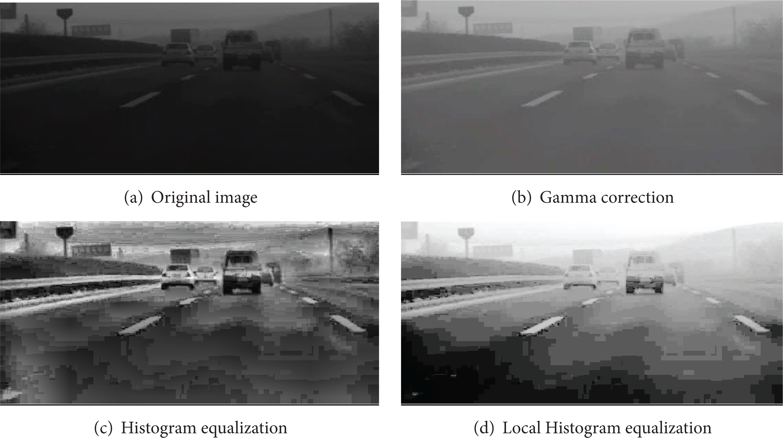
Different illumination normalization algorithm.
2.2. Geometry Normalization
In order to be suitable for the convolutional nets, images should be cropped to yield fixed size of 32*32. However, the problem of generalizing from nearby objects to far objects is daunting, because apparent size scales inversely with distance: size ∝ 1/distance, which may result in information incomplete in cropped subimage if we adopt the same size for cropping. Our solution is to create a normalized “pyramid” of five subimages that are extracted at geometrically progressing distances from the camera [1], as shown in Figure 2.

The image on top has been systematically cropped, leveled, and subsampled to yield each pyramid row seen at bottom. The bounding boxes demonstrate the effectiveness of the normalization.
Each subimage has the same pixel width but different pixel height after cropping and then they are scaled in different scaling ratio according to the experiment (details in Section 4). The scaling ratio of the farthest row is 1 and the others are all greater than 1.
3. Convolutional Neural Network
3.1. The Characteristics of Convolutional Neural Network
The convolutional neural network (CNN) combines three architectural ideas to ensure some degree of shift, scale, and distortion invariance: local receptive fields, shared weight, and spatial or temporal subsampling. The local receptive fields are trained to extract local features and patterns. The CNN uses weight sharing over the input areas, which naturally produces invariance to translation, scaling, and some rotation. The subsampling between convolutional layers increases the shift and scale invariance, while reducing computational complexity and the hierarchical architecture creates complex features. This architecture makes convolutional nets naturally shift and scale invariant and is therefore desirable for learning robust and discriminative visual features. Convolutional neural network, an effective recognition algorithm, is widely used in fields such as pattern recognition and image processing, and can be good at extracting with category implicit characteristics of the resolution.
3.2. The Structure of a Typical Convolutional Neural Network LeNet-5
A typical convolutional neural network named LeNet-5 is shown in Figure 3 as presented in [6]. The network comprises 7 layers, not counting the input, all of which contain trainable parameter. The input is a 32*32 pixel image. The convolutional layer is labeled C i , while the S i indexes the subsampling layer and F i denotes the full connection layer, where i is the layer index. Each layer contains one or more planes. Approximately centered and normalized images enter at the input layer. Each unit in a plane receives input from a small neighborhood in the planes of the previous layer.

Architecture of LeNet-5, a convolutional neural network. Each plane is a feature map.
Note that in case of a convolution, the size of the successive field shrinks because the border cases are skipped. For subsampling operations, a simple method is used which halves the dimensions of an image by summing up the values of disjunctive 2 × 2 subimages and weighting each result value with the same factor. The term “full connection” describes a function in which each output value is the weighted sum over all input values. Note that a full connection can be described as a set of convolutions where each field of the preceding layer is connected with every field of the successive layer and the filters have the same size as the input image [15]. For further details about LeNet-5, we recommend in Section 4.
4. Experiments
The completed recognition and classification process is shown in Figure 4.

The integrated process of traversability analysis of vehicles.
The preprocessing and normalization are accomplished in Section 2.
4.1. The Type and Structure of the Network
In this paper, the convolutional neural network, LeNet-5, is adopted and the unit number of output layer is adjusted to 3, which denots the vehicle and the roadside, respectively, and the road. Layer C1 consists of 6 feature maps, each unit in each feature map is connected to a 5*5 neighborhood in the input, so the size of every feature map of C1 is 28*28. Layer C1 contains 156 trainable parameters and 122,304 connections. The convolutional layer is described as

where l denotes the number of layer, k is the convolutional kernel, M j represents the chosen feature map, and b indexes the bias.
Layer S2 consists of 6 feature maps, each unit in each feature map is connected to a 2*2 neighborhood in the corresponding feature map in C1, so the size of every feature map of S2 is 14*14. Layer S2 has 12 trainable parameters and 5,880 connections. The subsampling layer is described as

where down (·) denotes the subsampling function and β and b is typical for every feature map.
Layer C3 consist of 1,516 trainable parameters and 151,600 connections. Layer S4 has 32 trainable parameters and 2,000 connections. Layer C5 contains 48,120 trainable connections. Layer F6 is fully connected with C5. After each layer a bias is added to every pixel (which may be different for each field) and the result is passed through a sigmoid function, for example, s(x) = a*tanh(b*x), to finally perform a mapping onto an output variable. The output consists of radial basis function (RBF) [11]. In order to be consistent with the three objects in front of the vehicle on the highway, we change the output number of the convolutional net to three. That is, our targets for identification and classification are three types, including the road, the vehicle, and the roadside.
4.2. Image Labeling
Firstly, for the grayscale image set P which is processed by the Gamma correction, the pixel points whose gray value equals to 0, as well as those whose gray value equals to 255, are adjusted to gray values between 0 and 255 by programming. Secondly, the gray value of the pixel points which represent the vehicle is set to 0 and the gray value of those which represent the roadside is set to 255, respectively. After all, an image set Q is obtained. Now, we get three types of pixel points which are given the corresponding labels respectively, including “0,” “1,” and “2.” Among them, the label “0” represents the road, the label “1” represents the vehicle, and label “2” represents the roadside. Finally, the pixel points belonging to the image set Q are given to the corresponding pixel points belong to images set P by programming. So far, we accomplish the image labeling.
4.3. Training and Testing Samples Set
In the previous work, the original images are pre-processed, normalized, and labeled. In order to acquire input images of the CNN, a suitable geometry normalization approach should be presented. As we have mentioned in Section 2.2, for the convolutional nets, images should be cropped to yield fixed size of 32*32. In this paper, we achieve this process by the following steps. Firstly, we acquire the original images on the highway. Secondly, in different pixel row, we measure the lane width pixel and the vehicle height pixel. We use Y w and Y h to denote them, respectively. These measured data are used to curve fitting to obtain the stoichiometric relation between the pixel row and the lane width pixel, another is between the pixel row and the vehicle height pixel, as shown in (3). Finally, the geometry normalization for the image set Q is accomplished. In this paper, we choose 4,000 sample images for training and 1,400 sample images for testing. Part of the training samples and testing samples are shown in Figure 5.
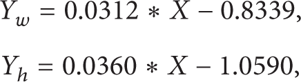
where X indexes the pixel row, Y w denotes the lane width pixel, and Y h is the vehicle height pixel.
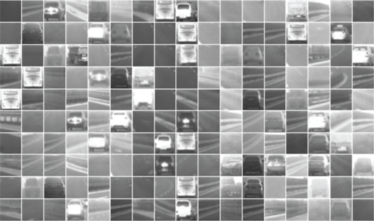
Part of the training samples and testing samples.
4.4. Training and Testing
The convolutional neural network is trained with the standard back-propagation algorithm. The targets are fixed to 0 for road, 1 for vehicle, and 2 for roadside. For testing, we adopt sample images different from the training samples to test the trained convolutional neural network at the number of 1,400. The training and testing process is shown in Figure 6.
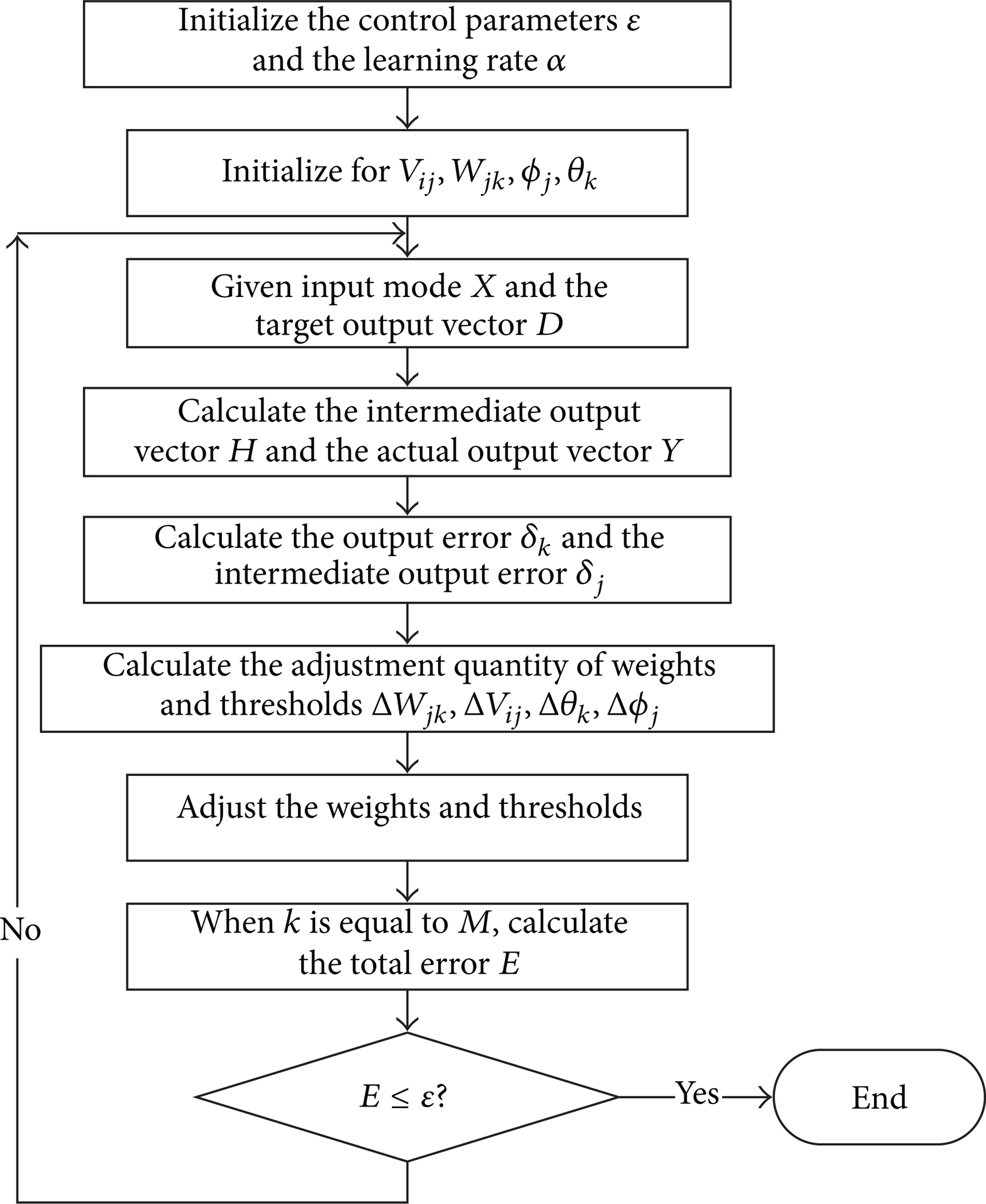
The flow chart of training and testing process.
4.5. Results
The root mean square error of training curve is shown in Figure 7, we can see that the mean square error becomes smaller and smaller as a whole, which indicates that the CNN has better performance. In the output of the testing, the color blue indexes the vehicle, yellow indexes the roadside, and red indexes the road.

The root mean square error of training curve.
In Figure 8, there are some areas that the CNN may recognize incorrectly; for example, the bottom of the vehicle may be recognized as the roadside and the lane may be misclassified as the vehicle, as shown in Figure 8 c3. In order to solve the problem, we can adopt better sample set to train the CNN, also we can adjust the masking method to recognize more correctly.
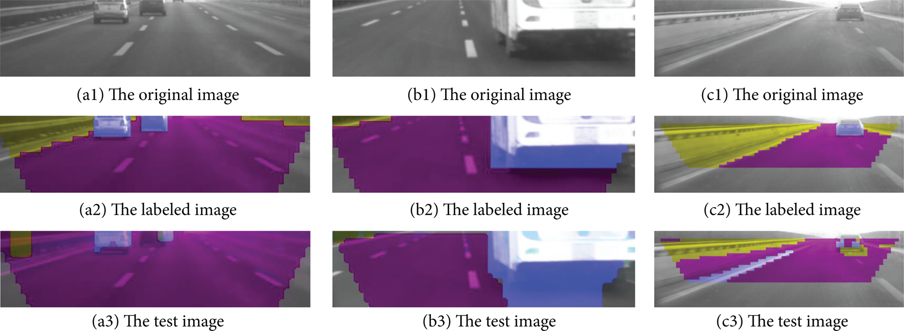
The testing results.
5. Conclusions
In this paper, the performance of the convolutional neural network, as the classifier in traversability analysis of vehicles on the highway, is proposed and tested The key technologies studied in this paper can be applied to vehicle safety, intelligent vehicle, auxiliary driving mobile robot, and so forth, to improve all kinds of onboard visual perception system of intelligent and the ability to automatically adapt to unknown environment and reflect the latest achievements of information technology with very high research value and broad application prospects.
The follow are further working we will study.
In order to research the traversability analysis of vehicles in other unknown environment, we will further study the structure and parameters of LeNet-5, we can adjust the unit number of output layers and feature map number of layer C5 to recognize and classify more objects accurately.
In next works, we will experiment with other and different types of convolutional neural network to test if there is a better convolutional neural network applied to traversability analysis of vehicles.
Conflict of Interests
The authors declare that there is no conflict of interests regarding the publication of this paper.
Footnotes
Acknowledgments
This paper is supported by the National Natural Science Foundation of China (Grant nos. 51107006 and 61203171), the China Postdoctoral Science Foundation (Grant no. 2012M510799) and the Fundamental Research Funds for the Central Universities (Grant nos. DUT12JS03 and DUT12JR04).