Hierarchical Spatial Clustering in Multihop Wireless Sensor Networks

Abstract

Wireless sensor networks have been widely deployed for environment monitoring. The resource-limited sensor nodes usually transmit the sensing readings to Sink node collaboratively in a multihop manner to conserve energy. In this paper, we consider the problem of spatial clustering for approximate data collection that is feasible and energy-efficient for environment monitoring applications. Spatial clustering aims to group the highly correlated sensor nodes into the same cluster for rotatively reporting representative data later. Through a thorough investigation of a real-world environmental data set, we observe strong temporal-spatial correlation and define a novel similarity measure metric to inspect the similarity between any two sensor nodes, which take both magnitude and trend of their sensing readings into consideration. With such metric, we propose a clustering algorithm named as HSC to group the most similar sensor nodes in a distributed way. HSC runs on a prebuilt data collection tree, and thus gets rid of some extra requirements such as global network topology information and rigorous time synchronization. Extensive simulations based on realworld and synthetic data sets demonstrate that HSC performs superiorly in clustering quality when compared with the alternative algorithms. Furthermore, approximate data collection scheme combined with HSC can reduce much more communication overhead while incurring modest data error than with other algorithms.

1. Introduction

In the recent years, wireless sensor networks (WSNs) have witnessed the wide utilization in environmental monitoring [1], for example, forest monitoring [2, 3], urban city monitoring [4], and office monitoring [5]. These WSNs typically consist of a huge number of tiny sensor nodes that are significantly short of available resources, especially the energy budget. These sensor nodes are usually organized as a multihop communication network and cooperatively transmit the sensing readings to the Sink node via a prebuilt data collection tree for the energy conservation purpose.

Longer network lifetimes of WSNs are always expected by the environmental monitoring applications. Reducing the communication overhead has been the uppermost principle for various algorithms in WSNs to prolong the network lifetime as wireless communication consumes the most energy among all the activities of a sensor node [6]. By exploiting the tradeoff between data quality and energy consumption, approximate data collection can be a rational choice for long term data-driven applications. It is argued that approximate data can still be precise enough for some applications, which can tolerate certain accuracy loss of sensing readings to perform data analysis or decision making [7]. Due to ubiquitous spatial correlation among nearby sensor nodes, some representative sensor nodes can be scheduled to transmit their readings to approximate the readings of their spatial correlated sensor nodes accordingly [8]. Spatial clustering, which combines the clustering technique and spatial correlation, becomes an effective approach to find these similar node sets, sensor nodes which can represent each other during data collection. Generally speaking, two core questions about spatial clustering are how to evaluate the similarity between data distributions of any two sensor nodes, and then how to group these similar sensor nodes into the same cluster in an energy-efficient manner. Previous works mainly measure the magnitude similarity with raw readings, but overlook the importance of trend similarity [8–11]. Yet, some work does exactly the opposite [12]. We argue that both magnitude similarity and trend similarity hold the equivalent importance. Due to the ad hoc nature and resource constraints of WSNs, distributed spatial clustering would be a better choice.

Through an investigation of a real-world environmental data set, we observe strong temporal and spatial correlation among sensor data. The spatial correlation makes spatial clustering feasible and necessary, while the strong temporal correlation implies the predictability of environmental data. We employ a time series analysis method, that is, Autoregressive (AR) model, to describe the predictable sensor data. An appropriate AR model can capture the reading trend of a sensor node in an easy way, and meanwhile two sensor nodes with similar reading trend tend to have the similar AR models. In this paper, we thus define a novel similarity measure metric which combines both magnitude similarity and trend similarity of sensor data by exploiting the AR models. With such metric, we propose the Hierarchical Spatial Clustering (HSC) algorithm to group the most similar sensor nodes. Based on the pre-built data collection tree, HSC can complete the clustering task gracefully without extra requirements, such as the global network topology information or rigorous time synchronization.

The contributions of this paper are summarized as follows.

• (i)

We have designed a novel sensor nodes similarity measure metric, which jointly takes magnitude similarity and trend similarity of sensor readings into considerations.

(ii)

With our similarity measure metric, we propose a hierarchical spatial clustering algorithm, that is, HSC, which effectively exploits the existing structure of multihop WSNs.

(iii)

We conduct extensive simulations based on both real-world and synthetic environmental data sets. The simulation results demonstrate the advantages of HSC on both clustering quality and clustering efficiency. Additional simulations on approximate data collection also prove the powerful approximation performance of HSC.

The rest of this paper is organized as follows. Section 2 discusses the related works. Section 3 presents the similarity measure metric. System model is described in Section 4, and the details of HSC are elaborated in Section 5. Section 6 presents the performance evaluation results, and Section 7 concludes this paper.

2. Related Work

In this section, we present and discuss the most related works on spatial clustering in WSNs. A well-reviewed survey of clustering algorithms in WSNs is referred to in [13]. As HSC relies on the AR model, we will also briefly review the related work of AR model in WSNs.

2.1. Spatial Clustering

Taking spatial and data correlation into account, spatial clustering aims to group sensor nodes with similar readings into the same cluster to capture the underlying spatial-temporal pattern in WSNs. Two key questions about spatial clustering are how to measure the similarity between readings of any two sensor nodes and how to group the sensor nodes with similar readings in an energy-efficient manner. Some previous works measure the similarity with raw readings based on Manhattan distance metric, mostly only on the magnitude similarity, such as DCglobal [9], DClocal [10], IADSC [14], DACA [15], and DSCC [16]. Similarity solely measured on magnitude similarity, however, cannot adapt to the dynamic of sensor readings caused by the dynamical environment [8]. Magnitude similarity only captures the temporal characteristic of sensor readings, but overlooks the possible changes in near future. Besides the magnitude similarity of raw readings, EEDC [8] also takes the trend similarity of sensor nodes into account. EEDC models the spatial clustering problem as a clique-covering problem which is proved NP-hard, and solves it with a greedy algorithm in a centralized fashion. In the scenario of centralized clustering, the Sink node needs to accumulate enough readings for each sensor node to perform similarity measure between any two sensor nodes. Obviously, the data accumulation procedure leads to huge communication overhead, and thus energy consumption. Even worse, spatial clustering may form “unsteady” spatial clusters if we measure the similarity of sensor nodes only on their raw readings.

ELink [12] emphasizes that spatial clustering should be performed on the underlying trend rather than on the raw time series sensor readings. According to ELink algorithm, each sensor node constructs an AR model to capture the structure of time series readings and computes its feature in the metric space of weighted Euclidean distance with the coefficients of AR model. Based on these features, ELink models the clustering problem as δ-clustering, where feature distance between any two sensor nodes in the same cluster is less than δ. Recursively, some well-distributed sensor nodes are chosen as sentinel nodes to expand their clusters until they are δ-compact in a distributed manner. Though taking the underlying trend of time series sensor readings into consideration, ELink overlooks the baseline value of each sensor node. In other words, sensor nodes in the same cluster could have the similar variation tendency, but their real sensing readings may differ greatly. Furthermore, the selection of the well-distributed sentinel nodes requires a priori global network topology information, meanwhile each sentinel node starts the clustering process relying on strict time synchronization. Both requirements on network topology information and time synchronization weaken the applicability of ELink in practice. SAF [11] also exploits the AR model when clustering. With the new concept of model clustering, SAF performs centralized clustering based on values predicted by AR models. SAF still only depends on the magnitude similarity of sensor nodes but leaves out the trend similarity. The centralized clustering manner also incurs amounts of communication overhead.

Different from the previous works, our algorithm, that is, HSC, takes both magnitude similarity and trend similarity of sensor readings into consideration, and groups the similar sensor nodes in a distributed and hierarchical manner based on a pre-built data collection tree with no other extra requirements on network topology information and time synchronization. Compared to the earlier version of HSC in [17], the new contributions of this paper includes the following. (i) Through an investigation of a real-world environmental data set in Section 3.1, we verify the feasibility of modeling sensor readings as AR model as well as the rationality and necessity of spatial clustering for approximate data collection. (ii) In Section 5.1, we formally define the spatial clustering problem in WSNs and prove the NP-hard of such problem. As an enhancement, we propose the cluster maintenance strategy for the spatial clusters to adapt to the dynamical environment in Section 5.3. We also analyze the message complexity and compatibility with other existing algorithms or protocols in WSNs of HSC in Section 5.4. (iii) More simulations are conducted to evaluate HSC in Section 6. The limitations and future works are also discussed in the conclusion section.

2.2. Autoregressive Model

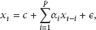
AR model is a linear regression, and is used to capture the dependency of current value and the latest historical values in time series data analysis. Readings of sensor nodes are obviously typical time series data, and the AR model can be adopted for data forecasting in WSNs. Though simple and light-weight, the AR model offers excellent accuracy in WSNs for monitoring applications [18, 19]. An AR model with order p, which is the number of lagged values in a linear regression, is usually denoted as AR(p), and expressed as

$$\begin{array}{cc}& x_t=c+\sum _{i=\mathrm{1}}^p‍{\alpha }_i{x}_{t-i}+ϵ,\end{array}$$

(1)

where $\overrightarrow{\alpha }=[{\alpha }_{\mathrm{1}},\dots ,{\alpha }_p]$ are the coefficients, c is a constant but always omitted for simplicity, and ϵ is the White Noise. The parameter estimation of AR model is quite simple, and various methods can be used. More details of AR model and time series data analysis are referred to in [20].

Due to low computation overhead and memory requirements yet outstanding performance in data forecasting, AR model has been widely used for approximate data collection in WSNs. PAQ [18] adopts AR model to approximate the values of sensor nodes. With AR model built locally, each sensor node transmits its model to Sink, which uses these models to predict values of sensor nodes without direct communication. PAQ proposes a dynamic AR model maintaining strategy to cope with the changing environment. With the dual-prediction based data collection idea in mind, quite a few similar works [7, 19] building on AR model have been presented, all of which adopt similar method to prolong the network lifetime of WSNs by keeping sensor nodes from transmitting redundant data. Besides exploiting AR model to model the temporal correlated sensor readings, HSC also takes advantages of spatial correlation among neighboring sensor nodes to group the similar nodes together, which would further reduce the energy consumption during data collection.

3. The Similarity Measure Metric

In this section, we will first investigate the environmental data features based on a real-world environmental data set, and then present our similarity measure metric which exploits such features.

3.1. Environmental Data Features

We mine the environmental data features with a real-world data set gathered by the Intel Berkeley Research Lab between February 28 and April 5, 2004. We refer to this data set as Intel data set. The Intel data set consists environmental data such as temperature, humidity, and light strength, which are collected by 54 Mica2Dot sensor nodes deployed in a $\mathrm{40}\hspace{0.17em}\text{m}\times \mathrm{30}\hspace{0.17em}\text{m}$ office. Specifically, we exploit the data of March 2004 to investigate the hidden characteristics of environmental data. The layout of the wireless sensor network and the data set can be found in [5].

In physical world, most types of environmental data, for example, temperature, humidity, and light strength, usually changes stably. It is considered that the difference between sensing readings of any sensor node in two consecutive time slots can be very small. Such feature of environmental data is normally referred as temporal correlation. To reveal this feature, we compute the absolute difference between readings of any two consecutive time slots for each sensor node across the entire month and plot the CCDF (Complementary Cumulative Distribution Function) results in Figure 1. Note that reading differences are processed with the min-max normalization method. From Figure 1, we observe strong temporal correlation existing in temperature, humidity, and light data. For any kind of environmental data, far less than $\mathrm{5}\%$ reading differences are greater than 0.1. This feature demonstrates that the environmental data indeed evolve stably and thus are predictable. Some probabilistic models are employed to capture the temporal correlation of environmental data for approximate data collection [18, 21, 22], among of which the AR model could be the most suitable one as mentioned in Section 2.2.

Figure 1

Temporal correlation in environmental data.

Another interesting feature about environmental data is that a small area in physical world generally shares a similar environmental condition. As a result, sensor nodes deployed closely would have similar sensing readings, and such phenomenon is referred as spatial correlation. To explore the spatial feature of environmental data, we compute the absolute reading difference between any two 1-hop neighboring sensor nodes, and plot the CCDF results in Figure 2. We simply set the transmission range to be $\mathrm{6}\hspace{0.17em}\text{m}$ to ensure good network connectivity by investigating the connectivity among sensor nodes. Each sensor node searches its 1-hop neighboring sensor nodes within such range. The data in Figure 2 are also the results processed with the min-max normalization method, and they show the strong spatial correlation of environmental data. In summary, only around $\mathrm{10}\%$ temperature and light reading differences are greater than 0.1, and less than $\mathrm{15}\%$ humidity reading differences is greater than 0.2. The spatial correlation feature of environmental data makes another form of approximate data collection possible that nearby sensor nodes can be represented by each other during data collection as their reading differences are negligible. Some approximate data collection methods have been proposed based on this feature, for example, [8–10]. Besides, the strong spatial correlation in WSNs is also the motivation for the spatial clustering algorithms.

Figure 2

Spatial correlation in environmental data.

3.2. Similarity Measure

In the context of approximate data collection, grouping sensor nodes with the most similar readings is of great importance. How to measure and distinguish such similarity between sensor nodes, however, is the first question we will face. As a concrete example, we have plotted 2000 temperature data of four sensor nodes, that is, sensor nodes 24, 25, 29, and 31 in the layout figure in [5], on March 9, 2004 in Figure 3. The humidity and light data have similar situations and are omitted here. From the figure, it is very intuitive for us to group nodes 24 and 25 together, and group nodes 29 and 31 together. We make such a decision mainly based on the observations from the magnitude and trend of the four data series. On the whole, nodes 24 and 25 have the most similar magnitude and varying trend. Same for the pair of nodes 29 and 31. However, relying on the first 500 data points, we may group the four nodes together when only considering their magnitude similarity. This simple example suggests that similarity measure on sensing readings of any two sensor nodes should take both the magnitude and trend into consideration.

Figure 3

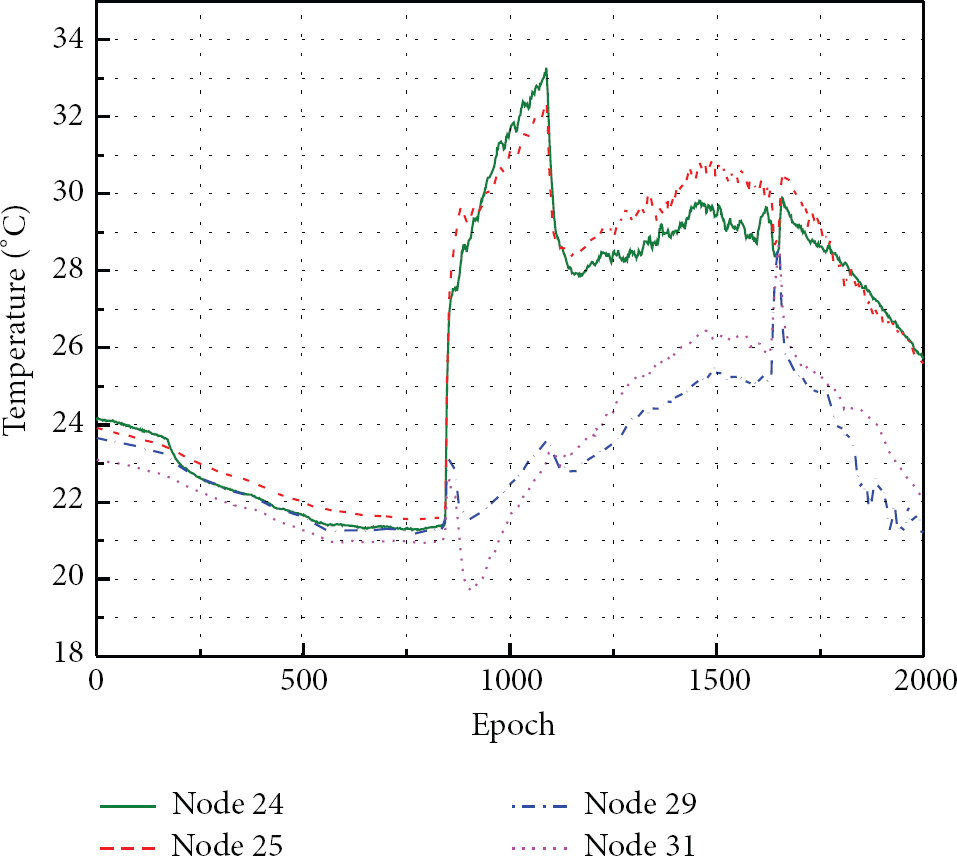
The evolution of temperature readings measured by four sensor nodes, that is, nodes 24, 25, 29, and 31 in the layout figure in [5].

As mentioned, we can adopt an AR model to capture the reading trend of a sensor node and measure the trend similarity of any two sensor nodes with their AR models. We would like to employ the average value μ of sensing readings of a sensor node in the past several time epochs to represent its corresponding magnitude situation. Thus, we can measure the magnitude similarity of two sensor nodes based on their average values rather than their raw readings to avoid amount of data exchanges during clustering. Consequently, it is feasible and reasonable to use the AR models and average values μ of any two sensor nodes to measure their similarity. On one hand, correlation between two AR models can be well measured with Pearson Correlation Coefficient. Formally, assuming two sensor nodes $s_i$ and $s_j$ with their AR(p) model coefficients $\overrightarrow{X}=[x_{\mathrm{1}},x_{\mathrm{2}},\dots ,x_p]$ and $\overrightarrow{Y}=[y_{\mathrm{1}},y_{\mathrm{2}},\dots ,y_p]$ , respectively, trend similarity between $s_i$ and $s_j$ can be calculated as

$$\begin{array}{cc}& {\rho }_{s_i,s_j}=\frac{\mathrm{cov}(\overrightarrow{X},\overrightarrow{Y})}{{\sigma }_{\overrightarrow{X}}{\sigma }_{\overrightarrow{Y}}}=\frac{E\left((\overrightarrow{X}-{\mu }_{\overrightarrow{X}})(\overrightarrow{Y}-{\mu }_{\overrightarrow{Y}})\right)}{{\sigma }_{\overrightarrow{X}}{\sigma }_{\overrightarrow{Y}}}.\end{array}$$

(2)

The greater ${\rho }_{s_i,s_j}$ , is the more the similarity between reading trends of $s_i$ and $s_j$ is. On the other hand, we adopt Manhattan distance to measure the magnitude similarity between their average values. If their magnitude similarity $M_{s_i,s_j}=|{\mu }_{s_i}-{\mu }_{s_j}|\le \epsilon /\mathrm{2}$ , then these two sensor nodes are considered magnitude similar, where ε is a user-defined parameter to bound the maximum difference between sensing readings of any two similar sensor nodes. Hence, we finally have the following metric to judge whether two sensor nodes are similar.

Definition 1 (similar nodes).

Two sensor nodes, $s_i$ and $s_j$ , are similar nodes (and thus can be grouped into the same cluster during spatial clustering) if their trend similarity ${\rho }_{s_i,s_j}\ge cth$ and magnitude similarity $M_{s_i,s_j}\le \epsilon /\mathrm{2}$ , where both $cth$ and ε are user-defined application-dependent parameters.

4. System Model

In this paper, we consider a WSN consisting of a collection $S=\{s_{\mathrm{1}},s_{\mathrm{2}},\dots ,s_N\}$ of N sensor nodes and one Sink node. All sensor nodes are uniformly and randomly distributed in a sensing field. A powerful Sink node is deployed to gather sensing readings from the whole network. All sensor nodes have the identical communication radius R and communicate with distant nodes hop by hop. Periodically, sensor nodes generate environmental readings which evolve over time, and transmit these readings to Sink node via a data collection tree (DCT). In the multihop scenario, a DCT is requisite and can be built in a distributed manner. For instance, by circulating a tree formation message originated by Sink and making use of a min-hop parent selection strategy or other algorithms used for constructing maximum-lifetime data gathering tree [23]. After building the DCT each sensor node learns its unique $dct\_parent$ node in the DCT, and maintains a list of its direct children nodes in DCT, $dct\_children$ .

Furthermore, each sensor node maintains a queue to store the most recent W sensing readings and keeps tracking of the average value μ of those W data. The size of data queue would not be very great so that no extra storage space is needed to add for current sensor node platform. By exploiting the readings in queue, each sensor node can learn an AR model using least-square method. Similar to PAQ [18], we also adopt a narrow prediction window, that is, $p=\mathrm{3}$ , to neglect the impact of non-stationary physical environment. This setting also makes the AR model simple and light-weight enough for resource-limited sensor nodes. To cope with dynamical environment, for example, the rapid temperature change around the 800th epoch in Figure 3, we adopt the model monitoring algorithm of PAQ to maintain an accurate and dynamic local AR model for each sensor node. A sensor node generally relearns its AR model using the latest W data in queue if the times of the prediction error beyond error threshold θ within consecutive Λ epochs exceeds a predefined threshold ν.

5. The Spatial Clustering Algorithm

5.1. The Spatial Clustering Problem

So far, we have presented an effective similarity measure metric to examine whether two sensor nodes are similar on the sensing reading distribution. In this subsection, we formally define the spatial clustering problem in the context of approximate data collection and propose a solution for the second core question, that is, how to energy-efficiently group the similar sensor nodes.

Definition 2 (spatial clustering problem).

For a multihop WSN with a collection $S=\{s_{\mathrm{1}},s_{\mathrm{2}},\dots ,s_N\}$ of N sensor nodes, the whole network can be partitioned into definite node sets $C=\{C_{\mathrm{1}},C_{\mathrm{2}},\dots ,C_y\}$ , where ${\bigcup }_{a=\mathrm{1}}^y{C}_a=S$ . For all $s_i,s_j\in C_a$ , $s_i$ and $s_j$ are similar nodes; that is, ${\rho }_{s_i,s_j}\ge cth$ and $M_{s_i,s_j}\le \epsilon /\mathrm{2}$ . Spatial clustering aims to group the similar nodes into the same cluster and meanwhile obtain $\min y$ .

There are actually two objectives for any spatial clustering algorithm. One is to ensure all sensor nodes in the same cluster are remarkably similar, and the other one is to minimize the number of such kind of clusters. The two objectives together guarantee the data accuracy and energy efficiency of approximate data collection. Unlike some algorithms which perform clustering first and then build the DCT, we argue that spatial clustering should not break the pre-built DCT structure as it may be built by some optimal algorithms, for example, [23]. Due to above considerations, spatial clustering is quite a challenging task. Interestingly, the spatial clustering problem can be modeled as a set-covering problem. We construct a graph G with sensor nodes as vertices. There is an edge $(s_i,s_j)$ , if $s_i$ and $s_j$ are similar nodes. Note that in the spatial clustering problem, an “edge” exists between two similar nodes directly or indirectly through several intermediate similar nodes. Finally, spatial clustering problem shares the same objective with the set-covering problem, that is, using the minimum clusters to cover all vertices in the graph G. The set-covering problem is known as an NP-hard problem [24], thus the spatial clustering problem could be proved as an NP-hard problem. For such tough task, we propose a spatial clustering algorithm called HSC based on the existing DCT.

5.2. The HSC Algorithm

The HSC algorithm includes two phases: the local AR model learning phase and the hierarchical spatial clustering phase, which are introduced in details as follows.

5.2.1. The Local AR Model Learning Phase

To avoid transmitting abundant raw readings to Sink node for model building, we prefer to learn and maintain the AR model locally at each sensor node. After accumulating enough data, that is, W data to feed the queue full, each sensor node will estimate the coefficients of AR( $\mathrm{3}$ ) model by calculating the minimum square error between the real readings contained in the queue of that sensor node and the predicted values via least-square regression method. Note that other parameter estimation methods for AR model, for example, maximum likelihood, could be used, but least-square regression could be a more proper method as it is simple enough to avoid complex computation.

5.2.2. The Hierarchical Spatial Clustering Phase

Once a sensor node completes the AR model learning phase, it then transmits the coefficient vector $\overrightarrow{\alpha }$ and the average value μ to the Sink node via DCT. During the parameters transmission, each intermediate node backups the average values of its direct children nodes in DCT and stores these values in buffer Γ. With all model coefficients transmitted to the Sink node, it facilitates the combination of HSC and the dual-prediction based approximate data collection schemes, which will be illustrated in Section 6. In principle, HSC is initiated by the Sink node and extended top down along with the DCT. During the execution of HSC, there are three primary roles for sensor nodes: trigger node, sentinel node, and expanding node.

Trigger Node. A trigger node selects the minimum number of sentinel nodes from its $dct\_children$ to cover all of its children nodes based on their average values stored in buffer Γ. Formally, a node $s_i$ is considered to be covered by another node $s_j$ if they are magnitude similar; that is, $M_{s_i,s_j}\le \epsilon /\mathrm{2}$ . To select as few sentinel nodes as possible, we adopt a median-value-first strategy. First, the node whose average value is the median value among all data in buffer Γ is chosen, and then those nodes whose average values are covered by the median value are sought out. If there are still some uncovered values, we repeat this strategy at the separated upper part and lower part uncovered values of the median value independently until all values can be covered by at least one sentinel node. This operation is performed among average values of nearby sensor nodes that share similar observations, thus the median-value-first strategy is feasible and can terminate quickly. At last, trigger node will transmit the complete selection result to all of its $dct\_children$ nodes.

Sentinel Node. A sentinel node will be the clusterhead of a spatial cluster. After being chosen as sentinel node by a trigger node, this sensor node broadcasts an Invitation message to its 1-hop neighbors. The message is encoded as $〈\overrightarrow{\alpha },\mu ,hops〉$ including the model coefficients $\overrightarrow{\alpha }$ , average value μ, and hop distance $hops$ from this sensor node to the Sink node; however, only the $dct\_children$ and sibling nodes of this sentinel node will respond to this Invitation message with feedback as either Join message or Reject message, depending on whether that sensor node is similar or dissimilar with current sentinel node. Sibling nodes are those nearby sensor nodes that have the same hop distance to the Sink.

Expanding Node. After receiving an Invitation message from a sentinel node, any sensor node $s_i$ will first check whether it is similar with that sentinel node on both aspects of magnitude and trend based on their $\overrightarrow{\alpha }$ and μ. If similar, $s_i$ becomes an expending node, and then forwards the Invitation message only to its children nodes in DCT to expand current spatial cluster. Otherwise, $s_i$ replies Reject message to that sentinel node immediately.

When the Sink node has received model coefficients and average values from all sensor nodes, it becomes the first trigger node and selects several sentinel nodes from its 1-hop neighboring sensor nodes. With no guarantee of strict time synchronization, HSC adopts the Request-ACK mechanism to ensure that every communication during clustering is complete. Spatial clustering iterates among sensor nodes top down along with DCT, and each sensor node replies to its $dct\_parent$ node with Reject message immediately or ACK message after it has received feedback messages, either Reject or ACK, from all of its $dct\_children$ . A sensor node, no matter sentinel node or expanding node, will switch to be trigger node when it finds that some of its $dct\_children$ are not similar with current sentinel nodes; namely, that node should select several new sentinel nodes from the unclustered nodes to continue the spatial clustering. A trigger node do not finish its duty until all of its $dct\_children$ are either sentinel nodes or clustered by a sentinel node.

Figure 4 shows a sample execution of HSC clustering with user-defined parameters $\epsilon =\mathrm{0.5}$ and $cth=\mathrm{0.9}$ . Box attached with each node describes the average value μ and correlation ρ with neighboring nodes of current node. Node $s_{\mathrm{1}}$ is selected as a sentinel node by its $dct\_parent$ and prepares to expand its cluster with Invitation messages disseminated down along DCT. Node $s_{\mathrm{2}}$ is similar to clusterhead $s_{\mathrm{1}}$ and becomes an expanding node to forward the Invitation to its $dct\_children$ . However, both $s_{\mathrm{4}}$ and $s_{\mathrm{5}}$ are dissimilar with current sentinel node, that is, $s_{\mathrm{1}}$ . After receiving the Reject messages from its $dct\_children$ , node $s_{\mathrm{2}}$ turns to be trigger node and selects $s_{\mathrm{5}}$ as the sentinel node from the unclustered set $\{s_{\mathrm{4}},s_{\mathrm{5}}\}$ with median-value-first strategy. Meanwhile, $s_{\mathrm{2}}$ sends ACK to $s_{\mathrm{1}}$ to affirm the cluster relation. With the assignment, $s_{\mathrm{5}}$ broadcasts Invitation messages to its 1-hop neighbors. As sibling node, $s_{\mathrm{4}}$ checks the message and finally accepts the invitation to expand this cluster. On the other hand, $s_{\mathrm{3}}$ rejects the invitation from $s_{\mathrm{1}}$ once it finds that it does not meet the conditions of similar nodes with $s_{\mathrm{1}}$ . As the only unclustered $dct\_children$ node, node $s_{\mathrm{3}}$ is acknowledged as sentinel node by node $s_{\mathrm{1}}$ to form another cluster. Similarly, spatial clustering is hierarchically performed among the remaining nodes. Finally, there are four clusters and nodes in each cluster form a cluster tree.

Figure 4

A sample execution of HSC clustering algorithm.

5.3. Cluster Maintenance

Due to dynamic of the monitored environment, it is possible that the similarity conditions among cluster members cannot hold any more. Generally, it is preferable to perform dynamic cluster maintenance rather than repetitively clustering the whole network. In fact, both update of AR( $\mathrm{3}$ ) and variation of μ may lead to a procedure of cluster maintenance. During cluster maintaining, the similarity between the variational node and the clusterhead should be verified using the conditions of similar nodes. Regarding nonclusterhead $s_i$ , it propagates message up the cluster tree to obtain the updated $\overrightarrow{\alpha }$ and μ of the clusterhead. With the new information, $s_i$ examines whether it is still similar the clusterhead. If not, node $s_i$ broadcasts a message to get information of nearby clusters and merges into a suitable one. At its worst, $s_i$ becomes a singleton cluster. When a clusterhead $s_{\text{ch}}$ has significant change on data distribution, $s_{\text{ch}}$ propagates an updating message, which contains the latest $\overrightarrow{\alpha }$ and μ values, down the cluster tree to all of its cluster members. With the new parameters, each cluster member decides whether to stay in or depart from this cluster, both depending on the similarity measure result with $s_{\text{ch}}$ . As time goes, it is foreseeable that there will be more and more clusters. To keep the cluster number small, the whole network needs reclustering when the number of clusters exceeds a threshold $\text{Ma}{\text{x}}_{\text{clusters}}$ .

To reduce the verification frequency of changing μ, the variation is considered significant only when it meets certain conditions. Let the average value ${\mu }_i$ at $s_i$ update to ${\mu }_i^{\prime }$ , and the average value of its clusterhead when clustering is ${\mu }_{\text{ch}}$ . Then, when μ of nonclusterhead node meets $|{\mu }_i^{\prime }-(|{\mu }_i^{\prime }-{\mu }_i|/{\mu }_i)\times {\mu }_{\text{ch}}|>\epsilon$ and μ of clusterhead meets $|{\mu }_i^{\prime }-{\mu }_i|>\epsilon$ , similarity verification between sensor nodes is necessary.

5.4. Discussion

Now we will discuss the communication overhead of our spatial clustering algorithm. Assume H clusterheads are finally selected. Specifically, $h_{\mathrm{1}}$ clusterheads are selected within the first round, and the others $h_{\mathrm{2}}=H-h_{\mathrm{1}}$ are selected among $m{h}_{\mathrm{2}}$ sensor nodes within extra rounds, where m is the average number of dissimilar sensor nodes during clusters expanding, far less than $(\pi R^{\mathrm{2}}/L^{\mathrm{2}})N$ . Therefore, H selection result messages, H ACK messages, and $m{h}_{\mathrm{2}}$ Reject messages are generated during clusterheads selection with 1 hop distance. In addition, H Invitation messages are sent out, following with $(N-H)$ Join messages. If we assume the average size of cluster trees is d hops, then there are totally $\mathrm{2}H+m{h}_{\mathrm{2}}+dH+d(N-H)<(m+\mathrm{2})H+dN$ data communication. With typical setting like Section 6.1 and the general clusterhead ratio of HSC (less than $\mathrm{5}\%$ as shown in Figure 7 with appropriate parameters), the total communication will be no more than $(d+\mathrm{1})N$ ; that is, the message complexity of HSC is $O(N)$ .

Compared with previous works, for example, ELink [12], the DCT structure liberates HSC from the requirements of global network topology information and strict time synchronization. HSC takes advantage of the DCT built by some optimal algorithms, but does not try to build the routing tree itself. Therefore, these features make HSC coexist well with other existing algorithms or protocols, such as data gathering tree constructing algorithms, for example, [23], or approximate data collection schemes, for example, [18].

6. Performance Evaluation

In this section, we evaluate the clustering quality of HSC with extensive simulations. We further explore the efficiency of HSC for approximate data collection on aspects of both energy efficiency and accuracy of collected data. Three alternative algorithms are implemented as contrasts, and the simulations are conducted on both real-world and synthetic environmental data sets.

6.1. Simulation Setup

6.1.1. Compared Algorithms

As emphasized in Section 2, two critical factors of spatial clustering are the similarity measure on data distribution of sensor nodes and the fashion to group similar sensor nodes. Accordingly, we select two noteworthy previous works, that is, EEDC and ELink, as the alternative algorithms. EEDC measures the similarity of sensor nodes on both magnitude and trend of raw sensor readings and groups similar nodes in centralized manner. ELink measures the sensor node similarity only on reading trend by exploiting the AR model coefficients and performs distributed clustering to group similar nodes. For fairness, we design a new compared algorithm named as μELink, which is modified based on ELink to consider the magnitude situation μ when measuring similarity of sensor nodes. In short, μELink measures the similarity of sensor nodes using our metric, while performing clustering following the way of ELink.

6.1.2. Evaluation Metrics

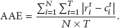
The quality of spatial clustering is measured by the number of generated clusters and the total number of communication messages used for spatial clustering. To examine the approximation performance of one spatial clustering, we evaluate the energy consumption and average absolute error (AAE) of collected data when the spatial clustering is combined with certain data collection scheme to conduct approximate data collection. In this paper, we substitute messages for energy consumption as data communication is the dominating energy consumer [6]. The AAE is calculated using (3), where $r_i^t$ and $c_i^t$ are the real value and the collected value through the approximate data collection scheme of sensor node $s_i$ at the tth epoch respectively, N is the total number of sensor nodes, and T is the total epochs of data collection. Consider the following:

$$\begin{array}{cc}& \text{AAE}=\frac{{\sum }_{i=\mathrm{1}}^N‍{\sum }_{t=\mathrm{1}}^T‍|r_i^t-c_i^t|}{N\times T}.\end{array}$$

(3)

6.1.3. Environmental Data sets

We have prepared two data sets (and thus different network models) for the simulations.

Real-World Data Set. We adopt the temperature data on March 9, 2004 of Intel data set mentioned in Section 3 as the real-world data set. Besides, the network model is designed following the layout shown in [5]. Fifty-foure sensor nodes are deployed in an office to persistently collect temperature readings with communication range R as $\mathrm{6}\hspace{0.17em}\text{m}$ . A Sink node is located at the center of the office to gather readings from all sensor nodes.

Synthetic Data Set. To evaluate the performance of HSC in larger scale scenarios, we design a hypothetical network model and the corresponding synthetic data set. N sensor nodes are deployed in a $\mathrm{100}\hspace{0.17em}\text{m}\times \mathrm{100}\hspace{0.17em}\text{m}$ field with identical communication radius $R=\mathrm{30}\hspace{0.17em}\text{m}$ . The Sink node is located at $(\mathrm{120}\hspace{0.17em}\text{m},\mathrm{50}\hspace{0.17em}\text{m})$ . We generate synthetic data set with similar method as DClocal [10]. Twenty-five event sources are fixed in the field in uniform distribution, and readings of sensor node are the comprehensive influencing results of all event sources. The influence of an event source to a sensor node is inversely proportional to the geographic distance between them. We employ the temperature data of Intel data set on March 9, 2004 to simulate the evolutive values of event sources. At the beginning of each simulation, we randomly select 25 data series from the 54 sensor nodes to map to the 25 event sources.

6.1.4. Parameters Setting

The size of the queue in each sensor node is set to be $W=\mathrm{60}$ , an appropriate value to produce a preferable AR model for environment monitoring [18]. For the monitoring algorithm of local AR model, we adopt similar parameters setting as PAQ [18]; that is, $\theta =\mathrm{0.03}$ , $\mathrm{\Lambda }=\mathrm{15}$ , and $\nu =\mathrm{8}$ . We also adopt the optimum parameters setting for the compared algorithms. Specifically, trend similarity threshold $t=\mathrm{80}\%$ and $gmax\_dst=\mathrm{3}\mathrm{\hspace{0.17em}\hspace{0.17em}}hops$ for EEDC. Regarding to ELink and μELink, we set weight vector $\overrightarrow{w}=(\mathrm{0.5,0.3,0.2})$ for the coefficients of AR( $\mathrm{3}$ ) model and fix the feature distance threshold $\delta =\mathrm{0.5}$ . All results in this section are the average values of 10 simulations.

6.2. Quality of Spatial Clustering

In this subsection, we study the impacts of system parameters, that is, user-defined error bound ε, correlation threshold $cth$ , and the network size N, on the clustering quality of HSC with comparisons to the three alternative algorithms. Fixing other parameters and setting $cth=\mathrm{0.9}$ for HSC, we first perform simulation with the real-world data set. Figure 5 shows the number of formed clusters of each algorithm when we vary ε from 0.1 to 1.0. Generally, the more stringent requirement on the data accuracy is (smaller ε), the more clusters will be generated. With a small ε, the number of clusters is more than 40 for most algorithms except ELink. As a complicated environment, an office may contain various heat sources, and thus many clusters are needed for approximate data collection. On the contrary, ELink produces the same number of clusters regardless of ε, which is unreasonable in real world. This is mainly because of the only consideration of reading trend when ELink measures the node similarity. Our algorithm offers reasonable results with respect to different application requirement on ε.

Figure 5

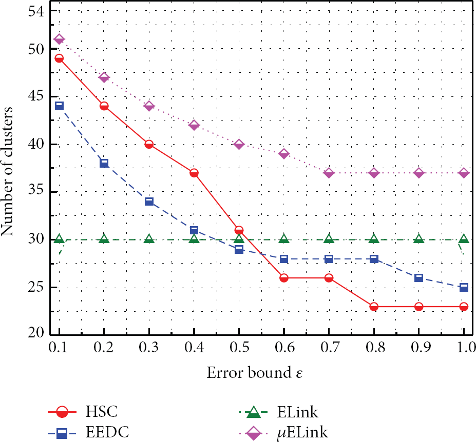
Impact of ε on clustering quality with real-world data set.

We also perform simulations on synthetic data set to evaluate the scalability of HSC. Figure 6 shows the number of total formed spatial clusters by each algorithm versus ε with a fixed network size $N=\mathrm{100}$ . When ε increases, the total cluster numbers of other three algorithms decrease except ELink. In most cases, HSC performs much better than the other algorithms. As ELink only takes the features calculated on AR model coefficients as the metric to measure similarity, the cluster number of ELink retains around $\mathrm{5}$ . Moreover, we study the clustering quality in various network sizes by varying N. With other parameters fixed as $\epsilon =\mathrm{0.5}$ and $cth=\mathrm{0.9}$ for HSC, we present the results in Figure 7. It is easy to understand that with the increase of N, the whole network will be partitioned into more clusters. HSC still generates much fewer clusters than EEDC and μELink and comparable quantity to ELink. As a matter of fact, merely considering the similarity on feature space but ignoring the magnitude similarity between sensor nodes, ELink has the loosest similarity requirements among all the four algorithms. Particularly, we perform experiments to study the impact of $cth$ on the clustering quality of HSC with ε fixed as $\mathrm{0.5}$ . Figure 8 shows that $cth$ does affect the clustering quality. Explicitly, with more rigorous correlation between sensor nodes during similarity measure in HSC, more clusters will be generated, and more communication messages are needed accordingly. Obviously, when $cth$ becomes greater, it will be more difficult for sensor nodes to be similar with each other, thus more clusters are needed to cover all sensor nodes.

Figure 6

Impact of ε on clustering quality with synthetic data set.

Figure 7

Impact of N on clustering quality with synthetic data set.

Figure 8

Impact of correlation threshold $cth$ on HSC clustering with synthetic data set.

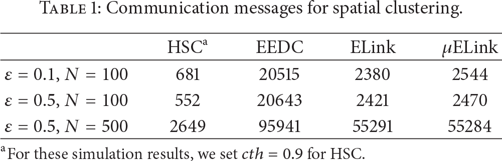
Regarding the communication messages for spatial clustering, Table 1 presents several brief results which are obtained with the synthetic data set. Undoubtedly, EEDC, due to transmitting all raw readings to the Sink node to perform centralized clustering, generates the most communication messages. Both ELink and μELink clustering are initiated by some well-distributed sentinel nodes, thus they need vast of messages to ensure communicating correctly in an asynchronous network. Note that it would also be quite difficult to find such kind of sentinel nodes in practice. Relying on the DCT, our algorithm starts from the Sink node and extends spatial clustering top down. It is illustrated as the results in Table 1 that HSC generates the minimum communication messages in various cases. The messages numbers also meet our approximate estimation $(d+\mathrm{1})N$ in Section 5.4, with different d in each case.

Table 1

Communication messages for spatial clustering.

	HSC	EEDC	ELink	μELink
$\epsilon =\mathrm{0.1}$ , $N=\mathrm{100}$	681	20515	2380	2544
$\epsilon =\mathrm{0.5}$ , $N=\mathrm{100}$	552	20643	2421	2470
$\epsilon =\mathrm{0.5}$ , $N=\mathrm{500}$	2649	95941	55291	55284

${}^{\text{a}}$ For these simulation results, we set $cth=\mathrm{0.9}$ for HSC.

6.3. Efficiency of Spatial Clustering

To examine the efficiency of spatial clustering, we have performed simulative approximate data collection via combining the four spatial clustering algorithms with certain approximate data collection schemes. In following simulations, we set parameters $\epsilon =\mathrm{0.5}$ , $cth=\mathrm{0.9}$ for HSC and perform $\mathrm{1000}$ epochs data collection for all algorithms based on the synthetic data set. For EEDC, we adopt the randomized intracluster scheduling and data restoration method [8] to perform approximate data collection. For the other three algorithms, we adopt the centralized model of PAQ [18] that is, the Sink predicts reading for each sensor node with values of its corresponding clusterhead, which sends periodic readings to Sink node. As shown in Figure 9, HSC and ELink consume much fewer communication messages for approximate data collection than the other two algorithms. Specifically, EEDC needs the most messages for data collection terms as the centralized algorithm EEDC needs all sensor nodes in the same cluster to transmit data to the Sink when it detects dissimilarity in that cluster. μELink consumes the most messages for clustering term, which includes messages for spatial clustering and cluster maintaining. Because of the introduction of average value and the distinctive distribution of clusters, μELink needs more messages to track the similarity between sensor nodes.

Figure 9

Communication messages for approximate data collection.

We plot a sample approximation result with HSC at a randomly selected sensor node in Figure 10. From this figure, we find that the real value and the approximated value are matched well. From the particular zooming-in results, we observe that the difference between the real value and the approximated value is negligible, which also demonstrates the excellent approximation performance of HSC. We also present the statistical results about collected data error of each algorithm in Table 2. EEDC has the smallest AAE due to its abundant data collection messages, and HSC takes the second place with a comparable result. Taking the average value μ into account, μELink surpasses ELink on this metric at the cost of huge cluster maintaining messages. In summary, HSC has much better comprehensive performance on the efficiency of data approximation than the other three algorithms.

Table 2

Average Absolute Error.

	HSC	EEDC	ELink	μELink
AAE	0.082	0.081	0.132	0.103

Figure 10

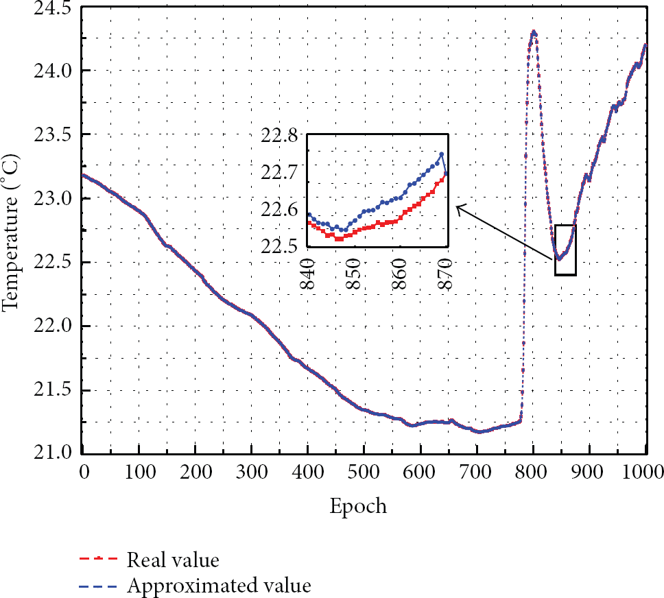
A sample approximation result of a randomly selected sensor node using HSC.

7. Conclusion and Future Work

Taking the AR model coefficients as an important clustering parameter, we design a novel similarity measure metric which gives coequal consideration to both magnitude similarity and trend similarity. With such metric, the proposed HSC algorithm groups the most similar sensor nodes based on DCT in a distributed manner. Extensive simulations are conducted with typical data sets, and the results shows the superior clustering quality of HSC when compared with three alternative algorithms. Furthermore, simulations based on an approximate data collection scheme demonstrate the efficiency and accuracy of our algorithm in data collection.

Currently, we only consider the environmental data, for example, temperature, humidity, and light strength, which are quite stable. WSNs have been used in various application domains and in each domain the sensing readings have different features; for example, the seismic signal data in volcano monitoring applications are high rate and can be sparsely represented in the wavelet domain [25]. As a matter of fact, HSC is more suitable in the scenario of environmental data collection, and some adaptive modifications should be done when migrating for other applications. In this paper, we consider both similarity measure metric and spatial clustering for the purpose of approximate data collection. In the future, we actually can extend such ideas to other research directions, and here are some possible future works. Firstly, we can borrow the idea of similarity measure of nodes for the sensor placement problem. In this problem, the deployment points correspond to the positions of clusterheads which are the most informative. Secondly, based on the formed spatial clusters, we could design some data aggregation algorithms to obtain the approximate reply for a statistic query, for example, MAX, MIN, and MEAN. Thirdly, some distributed decision making schemes could also be designed for event detection in WSNs based on the formed spatial clusters.