Sage Journals: Discover world-class research

Abstract

Direct numerical simulation has been performed to study a polymer drag-reducing channel flow by using a discrete-element model. And then, wavelet analyses are employed to investigate the multiresolution characteristics of velocity components based on DNS data. Wavelet decomposition is applied to decompose velocity fluctuation time series into ten different frequency components including approximate component and detailed components, which show more regular intermittency and burst events in drag-reducing flow. The energy contribution, intermittent factor, and intermittent energy are calculated to investigate characteristics of different frequency components. The results indicate that energy contributions of different frequency components are redistributed by polymer additives. The energy contribution of streamwise approximate component in drag-reducing flow is up to 82%, much more than 25% in the Newtonian flow. Feature of turbulent multiscale structures is shown intuitively by continuous wavelet transform, verifying that turbulent structures become much more regular in drag-reducing flow.

1. Introduction

It is well known that the addition of a small amount of polymer solution into liquid such as water at high Reynolds number can suppress turbulence and significantly reduce turbulent friction drag. This phenomenon, the so-called Toms effect [1], is useful for saving energy in turbulent flow systems and has recently been implemented in several industrial systems for energy conservation and environmental protection [2 –4]. The mechanism of drag reduction induced by polymer has been studied for several years, but there is still an absence of a widely accepted theory.

In the latest 20 years, along with the development of computer, more and more researchers studied the mechanism of polymer drag reduction by DNS. Sureshkumar et al. [5] performed DNS for a fully developed turbulence channel flow with FENE-P model and proposed a set of criteria for the onset of drag reduction. Dimitropoulos et al. [6] predicted drag reduction for a variety of rheological parameters in the FENE-P and the Giesekus models, and verified the hypothesis that one of the prerequisites for the phenomenon of drag reduction is sufficiently enhanced extensional viscosity, corresponding to the level of intensity and duration of extensional rates typically encountered during the turbulent flow. Angelis et al. [7] further confirmed the ability of the FENE-P model to reproduce most of the essential effects of polymers in dilute solutions on the wall turbulence. Min et al. [8, 9] studied the role of elastic energy in turbulence drag-reduction caused by polymer additives using an elastic Oldroyd-B model and obtained the maximum drag-reduction rate, showing good agreement with Virk's asymptote at the same Reynolds number. Ptasinski et al. [10] performed an analysis of the turbulent kinetic energy budgets and found that the ability of polymers to stretch is an essential ingredient for high drag reduction. Yu and Kawaguchi [11] studied the effect of Weissenberg number on the turbulent flow structure using a Giesekus model. Housiadas et al. [12] examined the efforts of changes in the flow viscoelasticity and the friction Reynolds number on several higher order statistics and on coherent structures of turbulence. Kajishima and Miyake [13] established a discrete-element model (spring-dumbbell model) to simulate the extension of polymer chain in drag-reducing flow. Then, this model was employed by Wang et al. [14] to investigate the mechanism of drag reduction by polymer. The decrease of the Reynolds shear stress found in the experiments was first reproduced in the simulation when the spring coefficient is relatively small.

However, most of the investigations mentioned above paid more attention to turbulent statistics relating to mean features of drag-reducing flow rather than different scale structures. Wang et al. [15, 16] attempted this topic especially for drag-reducing flow and its heat transfer by proper orthogonal decomposition. To make a further study on mechanism of drag reduction, multiresolution analysis method should be applied to investigate the energy distribution and turbulent structures of different time scales in drag-reducing flow. Fortunately, wavelet analysis theory provides an effective tool for detecting multiscale flow structures in turbulence. This theory is more and more widely used to analyze a series of turbulent phenomena such as atmosphere, ocean, river, and cloud [17 –20].

The first idea to use the wavelet analysis for studying turbulence was proposed by Farge [21] and some tools such as local intermittency and energy of wavelet decompositions, wavelet power spectrum, were developed to examine the structure of atmospheric turbulence. Camussi and Guj [22] conducted the wavelet decompositions with orthogonal-based wavelets to permit the identification of time signal series of coherent structures in artificial turbulence. Gilliam et al. [23] further verified that wavelet analysis can be employed to detect coherent structures in long-time series and introduce two statistical techniques, an intermittency rate estimator and an event-counting technique based on wavelet analysis to extract coherent structures from experimental data of wind. Smith and Jonas [20] proved that wavelet analysis is a useful tool for analyzing the turbulent data in cirrus clouds and found that wavelet spectra not only can be used to identify processes which produce energy at larger scales but also have the additional advantage to capture smaller-scale localized processes containing high-energy events along with their position in the time series, which may be lost in Fourier spectra obtained from long-time signals. Farge et al. [24] introduced a wavelet-based coherent vortex extraction technique for two-dimensional flows using scalar-valued orthogonal wavelet decompositions and decompose, turbulent flows into two orthogonal parts: a coherent, inhomogeneous, non-Gaussian component and an incoherent, homogeneous, Gaussian component, which have different correlations, different probability distributions, and different scaling laws. And then, this technique was extended to three dimensional conditions [25]. Based on wavelet, a new method called coherent vortex simulation was designed to model three-dimensional turbulent flows [26 –29]. Wavelet can also extract the characteristics of turbulence or eddy structures from experimental or computational data [30 –35]. Zhen and Hassan [36] applied wavelet analysis to the streamwise fluctuating velocity fields in the microbubbles drag-reducing flow for multiscale study and overcome many shortcomings of the Fourier analysis. In addition, wavelet analysis has been applied successfully in mechanics and chemical engineering for they provide both time and frequency information that helps in the industrial design of vessels and pipes [37, 38].

In the present study, the instantaneous information of polymer drag-reducing flow is provided by direct numerical simulation with the discrete-element model. Based on these DNS data, multiresolution structures of drag-reducing flow are analyzed by wavelet transformation and wavelet decomposition in time domain. Characteristics of different frequency components of time traces, such as wavelet energy spectra, intermittent factor, and intermittent energy, are examined by wavelet multiresolution decomposition to identify the polymer effect on turbulent energy distribution. Multiscale flow structures of Newtonian flow and drag-reducing flow are shown by continuous wavelet transform, respectively.

2. Physical Model and Numerical Method

In this study, the discrete-element model established by Kajishima and Miyake [13] is employed to simulate the polymer drag-reducing flow. The polymer chain is treated as a discrete-element and the polymer macromolecule is modeled as two beads linked by a spring and a damper as shown in Figure 1. The parameters in this model such as the spring coefficient k, damping coefficient η, and length l₀ represents elasticity, viscosity, and the natural length of the polymer chain, respectively. There are some assumptions introduced in the model: (1) the mass of the polymer is concentrated on the beads p and q, (2) linear transformation but not broken of spring, (3) the density of the discrete-elements equal to the solvent, (4) elastic collision between the beads and the wall, (5) ignore the interaction among the discrete-elements, (6) ignore the Brownian motions. Based on the assumptions mentioned above, the drag-reducing flow by polymer can be described as a sort of “two-phase” flow, a kind of liquid containing a large amount of discrete elements.

Figure 1:

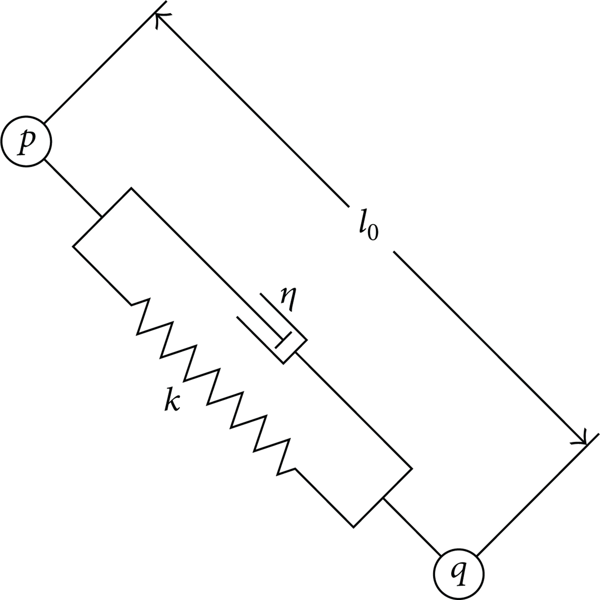
The discrete-element model.

DNS is performed for turbulent channel flow as shown in Figure 2. The dimensionless governing equations [14] for fully developed turbulent drag-reducing channel flow based on the discrete-elements model can be written as follows.

Figure 2:

Drag-reducing channel flow by polymer.

Discrete-elements motion equation:

\begin{matrix} \frac{d v_{p i}^{+}}{d t^{*}} = \frac{f_{p i}^{*} - k^{*} ξ^{*} ((x_{p i}^{*} - x_{q i}^{*}) / l^{*}) - η^{*} (v_{p i}^{*} - v_{q i}^{*})}{V^{*}}, \\ f_{p i}^{*} = - C^{*} (v_{p i}^{+} - u_{p i}^{+}) . \end{matrix}

(1)

For the solvent:

continuity equation:

\frac{\partial u_{i}^{*}}{\partial x_{i}^{*}} = 0,

(2)

momentum equation:

\frac{\partial u_{i}^{*}}{\partial t^{*}} + \frac{\partial}{\partial x_{j}^{*}} (u_{i}^{*} u_{j}^{*}) = δ_{i 1}^{*} - \frac{\partial p^{*}}{\partial x_{i}^{*}} + \frac{1}{R e_{τ}} \frac{\partial^{2} u_{i}^{*}}{\partial x_{j}^{*} \partial x_{j}^{*}} + F_{i}^{*},

(3)

additional force equation:

F_{i}^{*} = - \frac{1}{V_{c}^{*}} \sum_{x_{p}^{*} ∊ V_{c}^{*}} f_{p i}^{*},

(4)

where $k^{*} = k / ρ u_{τ}^{2} h$ , $η^{*} = η / ρ u_{τ} h^{2}$ , $C^{*} = 6 π r^{*} / R e_{τ}$ , $R e_{τ} = ρ u_{τ} h / μ$ , $u_{i}^{*} = u_{i} / u_{τ}$ , $x_{i}^{*} = x_{i} / h$ , $r^{*} = r / h$ , $t^{*} = t / (h / u_{τ})$ , $p^{*} = p / ρ_{f} u_{τ}^{2} + x^{*}$ , V^* = 4πr^*3/3, and V_c^* = V_c/h³.

The initial state of discrete-elements is assumed to be uniformly distributed in the solvent. The number of the elements is 10⁵. The dimensionless parameters r^*, l₀^*, k^*, and η^* are 0.01, 0.13, 0.001, and 0.0013, respectively. Calculations are made for a friction Reynolds number Re_τ = 150, which is based on the wall friction velocity u_τ and half the channel height h. The dimensionless computational domain 7.5 × 2 × 2.5 in the streamwise, wall-normal, and spanwise directions, respectively, is chosen, as shown in Figure 2. A grid system of 64 × 64 × 64 (x × y × z) meshes is adopted. The dimensionless time step 10⁻⁴ is used. The periodic boundary conditions are imposed in both the streamwise and the spanwise directions, while nonslip boundary conditions are adopted for the walls.

The Euler-Lagrange two-way method [39, 40], by which the motion of each element is tracked independently, is applied to obtain the distribution of discrete elements in drag-reducing flow. In this method, trajectories of elements' motion are obtained by solving the Newton equations of motion in Lagrange frame of reference. The computational algorithm is a fractional step method using the Adams-Bashforth scheme for time advancement [41] with the dimensionless time step 3 × 10⁻⁴ to solve velocities of solvent and beads. An implicit projection method is used for coupling velocity and pressure. Crank-Nicolson scheme is used for calculating the instantaneous locations of the beads. In discrete elements motion equation, the fluid velocity at the location of the beads is obtained by bilinear interpolation.

3. Wavelet Analysis

Wavelet transform is local transform revealing information in both the frequency and time domain. Continuous wavelet transform (CWT) of a given time series s(t) is defined as a convolution operation between the time series s(t) and a wavelet function ψ_{a, b}(t) as follows:

\begin{matrix} CW T_{s} (a, b) = 〈 s, ψ_{a, b} 〉 = \int_{R} s (t) \cdot ψ_{a, b} (t) d t \\ ψ_{a, b} (t) = \frac{1}{\sqrt{a}} ψ (\frac{t - b}{a}), \end{matrix}

(5)

where ψ_{a, b}(t) is wavelet function at translation b and scale a of the basic wavelet function ψ(t), also known as the mother wavelet.

Discrete wavelet transform is defined as following:

\begin{matrix} DW T_{a, b} = a^{- 1 / 2} \cdot Δ t \cdot \sum_{R} s (t) ψ (\frac{t - b}{a}) \\ = {a_{0}}^{- m / 2} \cdot Δ t \cdot \sum_{R} s (t) ψ ({a_{0}}^{- m} t - n b_{0}), \end{matrix}

(6)

where a = a₀^m, b = nb₀a₀^m, Δt = a^mb₀. a₀, and b₀ are the scale and time translation of wavelet function in first-level wavelet transform.

The original signal s(t) can be decomposed into n + 1 parts by n-level wavelet decomposition, including an approximate component A_n and n detailed components D_i shown as follows:

s (t) = A_{n} + \sum_{i = 1}^{n} D_{i} .

(7)

The energy E_{a, b} in the sense of time translation b and for scale a can be approximated by square of wavelet transform coefficients:

E_{a, b} = {| DW T_{a, b} |}^{2} .

(8)

Therefore, the total energy of scale a can be calculated as follows:

E_{a} = \sum_{b}^{} {| DW T_{a, b} |}^{2}, a = A_{j}, D_{j}, D_{j - 1}, \dots, D_{2}, D_{1} .

(9)

Energy contribution of different frequency (or scale) component is defined as the ratio between the energy of each level and total energy as follows:

E C_{a} = \frac{E_{a}}{\sum E_{a}}, a = A_{j}, D_{j}, D_{j - 1}, \dots, D_{2}, D_{1} .

(10)

Intermittency factor of components from wavelet decompositions is defined as a ratio between the number of higher energy events over energy threshold (I_{a, b} = 1) and total signals (N_a), which is written as follows:

\begin{matrix} I F_{a} = \frac{\sum_{b = 1}^{N_{a}} I_{a, b}}{N_{a}}, \\ I_{a, b} = {\begin{cases} 1, & DW T_{a, b} > th (a), \\ 0, & others . \end{cases} \end{matrix}

(11)

The energy threshold is defined as twice the average energy of that scale [21, 42]:

th (a) = 2 \overset{—}{E_{a, b}} .

(12)

Intermittent energy is defined as energy percentage of higher energy events in wavelet decompositions over their total energy as follows:

I E_{a} = \frac{\sum E_{a, b (I_{a, b} = 1)}}{E_{a}} .

(13)

For wavelet analysis, 6000 snapshots of velocity are selected and the interval dimensionless time is 3 × 10⁻².

4. Results and Discussions

Time and space averages of turbulent statistics in fully developed condition should be selected to obtain the mean flow field. It is written as follows:

\overset{—}{F (y^{*})} = \frac{1}{N_{x} \cdot N_{z} \cdot N_{t}} \sum_{i = 1}^{N} F (x^{*}, y^{*}, z^{*}, t_{i}^{*}) .

(14)

The fluctuating field can be calculated from the instantaneous field and the mean field as follows:

F^{'} (x^{*}, y^{*}, z^{*}, t^{*}) = F (x^{*}, y^{*}, z^{*}, t^{*}) - \overset{—}{F (y^{*})} .

(15)

Intensity of turbulent fluctuation is defined as the root mean square of the fluctuations [16]:

F_{rms} (y^{+}) = \sqrt{\frac{[\sum_{m = 1}^{N_{t}} \sum_{k = 1}^{N_{z}} \sum_{i = 1}^{N_{x}} F^{'} {(x_{i}^{+}, y^{+}, z_{k}^{+}, t_{m}^{*})}^{2}]}{(N_{x} \cdot N_{z} \cdot N_{t})},}

(16)

where y⁺ is the wall unit (y⁺ = (1 + y^*) · Re_τ) and F_rms(y⁺) represents instantaneous physical field such as fluctuating velocity and vorticity. Drag reduction rate is defined as the reduction of the friction factor with respect to the Newtonian fluid at an equal mean Reynolds number [43]:

DR % = \frac{C_{f Dean} - C_{f}}{C_{f Dean}} \times 100 %,

(17)

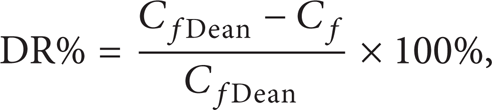
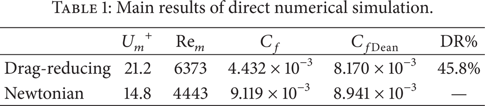
where DR% is the drag-reduction rate, C_f is the friction factor from DNS data and C_fDean is the friction factor of Newtonian fluid flow evaluated by Dean's correlation at the same mean Reynolds number of drag reducing flow. The main results such as frictional factor and drag reduction rate are listed in Table 1.

Table 1:

Main results of direct numerical simulation.

	U _m ⁺	Re _m	C _f	C _{f Dean}	DR%

Drag-reducing	21.2	6373	4.432 × 10⁻³	8.170 × 10⁻³	45.8%
Newtonian	14.8	4443	9.119 × 10⁻³	8.941 × 10⁻³	—

The mean velocity profile is shown in Figure 3. It can be seen that the mean velocity is in good agreement with linear distribution U⁺ = y⁺ in the viscous sublayer. In the buffer layer, mean velocity of drag-reducing flow increases significantly compared to those of Newtonian fluid flow.

Figure 3:

Mean velocity profile.

Figure 4 shows the velocity fluctuation intensities in the streamwise, wall-normal, and spanwise directions, respectively. The streamwise velocity fluctuation intensity of drag-reducing flow becomes larger than Newtonian fluid flow and its peak value position shifts to the bulk flow region. The other two components of velocity fluctuation intensities are depressed by drag-reducing additives, especially in the buffer layer. All the results mentioned above support that the buffer layer is the most effective region for drag-reducing additives to induce drag reduction.

Figure 4:

Velocity fluctuation intensities.

Turbulent statistics show the mean characteristics of flow. However, they cannot provide details of turbulent structure. In fact, turbulence is a very complicated phenomenon, which contains many multiscale structures in both time and space domain. Turbulent fluctuation consists of many different frequency components, of which large-scale structures represent low-frequency component of fluctuation in time series, while small-scale structures represent high-frequency component. Further investigation of the variation of different scale structures induced by polymer, multi-scale wavelet decomposition is employed to decompose the time series of velocity signals at a typical point into approximate component (A) and detailed components (D). In this paper, a typical point in the buffer layer (y⁺ = 15) is chosen for wavelet analysis because polymer plays a very important role in the buffer layer where peak values of important turbulent statistics and the maximum elongation of polymer molecules occur [16]. Then, the original velocity fluctuation signal u(t) can be decomposed into ten parts by nine-level wavelet decompositions (7) with 3rd order Daubechies wavelet.

Figure 5 shows the nine-level wavelet decompositions of velocity fluctuation. In these pictures, the first lines are time series of instantaneous velocity, and the others are different frequency components obtained from wavelet decompositions. From the 2nd line (A₉) to the 11th line (D₁), the frequencies of the components get higher and higher. It is obvious that the lowest frequency component (the 2nd line) can approximate the main features of the instantaneous velocity, which is in correspondence with the whole variation tendency of the local mean velocity along with time. And the higher frequency components can describe the details of turbulence, which reflect the occurrence of turbulent events. Comparing streamwise velocity components of Newtonian flow (Figure 5(a)) with drag-reducing flow (Figure 5(b)), it can be seen that the approximate component of the drag reducing flow has larger amplitude than that of Newtonian fluid flow (the amplitude is – 4 ∼ 2 for Newtonian fluid flow as A₉ of Figure 5(a) and – 5 ∼ 5 for the drag reducing flow as A₉ of Figure 5(b)). For Newtonian fluid flow, the detailed components show continuous stronger fluctuation along with time. The detailed components of the drag reducing flow show regular intermittent pulse as comparative weak fluctuation between every two strong fluctuations. All components of fluctuations of drag reducing flow show regular intermittence, indicating more regular burst events as compared with those of Newtonian fluid flow. Further explanations about these phenomena will be made later.

Figure 5:

Wavelet decompositions of the fluctuating velocity time series at the center point of the x-z plane at y⁺ = 15.

In order to further explain the polymer effect on velocity fluctuation, the energy contribution of different frequency components is calculated. Figure 6 shows the wavelet energy spectra of different levels from velocity decomposition. It is obvious that energy distribution of different frequency components has been changed in three directions by polymer additives. In partiular for the components in streamwise direction (Figure 6), there are remarkable differences in energy contribution between Newtonian fluid flow and drag-reducing flow. The energy contribution of approximate component (A₉) in drag-reducing flow is up to 82%, which is much higher than that of Newtonian flow 25%. For detailed components (D₉ ∼ D₁), the energy contributions of D₉ ∼ D₄ of drag-reducing flow are much less than those of Newtonian flow. These results show that energy of streamwise velocity is concentrated to the lowest frequency component and decrease in detailed components of drag-reducing flow, indicating that the energy redistribution induced by polymer makes the lowest frequency component have more significant effect on drag-reducing flow than on Newtonian flow. These conclusions are also in accordance with Figure 5 that the amplitude of streamwise approximate component becomes larger but almost all the amplitudes of streamwise detailed components get smaller in drag-reducing flow. On the other hand, the decrease of energy contributions of detailed components, which have a close relationship with turbulent dissipation, implies that there is a less energy loss in turbulent dissipation of drag-reducing flow, which may be another reason for drag reduction. It can be also found that polymer has a very weak effect on D₃ ∼ D₁ because these higher frequency components have smaller intensity so that they conclude tiny energy.

Figure 6:

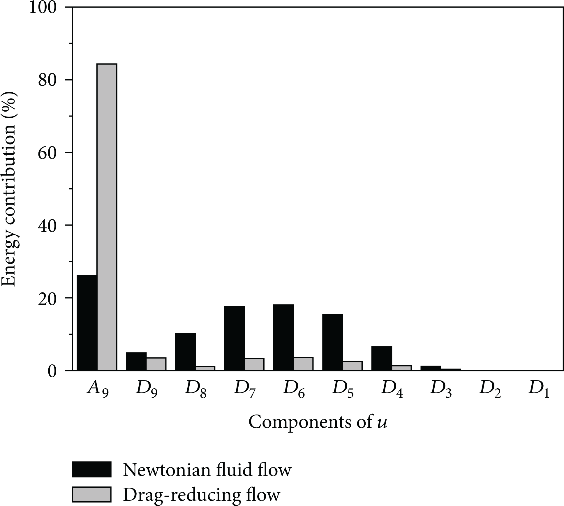
Energy contributions of different frequent components.

Intermittent factor and intermittent energy of different velocity components are shown in Figures 7 and 8, respectively. It can be seen that most energy is contained in high-energy events, a minority of all turbulent events. In drag-reducing flow, the intermittent factor of approximate component of streamwise velocity is about 20% but the intermittent energy is close to 65%. The intermittent factor and intermittent energy of approximate component (A₉) of drag-reducing flow are higher than those of Newtonian fluid flow, indicating that the number of high energy events of approximate component increases, intermittency strengthens, and more turbulent kinetic energy concentrates on high energy events in drag-reducing flow. High-energy burst events play a leading role in the formation of turbulent coherent structure. That is, stronger intermittency leads to larger-scale structures and more regular flow. Therefore, energy concentration on high-energy events signifies that turbulences are controlled and become more regular in drag-reducing flow. Moreover, intermittent factors of detailed components in drag-reducing flow are smaller, but intermittent energy is larger than those in Newtonian fluid flow, implying that the number of high energy events of detailed components decrease but turbulent kinetic energy of small scale structures remain concentrating on high energy events in drag-reducing flow. These support that turbulent events become more regular in drag-reducing flow. The conclusions from these two figures are also agree well with Figure 5 that number of larger amplitude of detailed components decrease and turbulent burst events appear more regular in drag-reducing flow.

Figure 7:

Intermittent factors of different frequent components.

Figure 8:

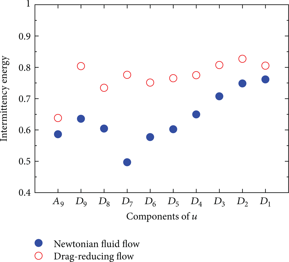
Intermittent energy of different frequent components.

Continuous wavelet transform with Morlet wavelet is used to investigate the influence of drag-reducing additives on turbulent multiscales structure. The continuous wavelet transform coefficients of instantaneous velocity time traces are shown in Figure 9. The lighter color indicates the larger wavelet transform coefficients, which means an intense turbulent event of time scale a occurs at time position b. On the contrary, the darker color indicates the smaller wavelet transform coefficients. In addition, the wider the coefficient streak along time axis (horizontal axis) is, the larger the scale of the structure is. From Figure 9, it can be found that when the time scale (vertical axis) decreases, the coefficient streaks become slimmer and their number increases exponentially. When time scale a decreases to less than about 25, coefficient streaks break down and several points with light or dark color appear. These phenomena intuitively show that turbulence is composed of many different scale structures. Obviously, coefficient streaks of Newtonian flow have more furcations. Nevertheless, drag-reducing flow has more regular and wider coefficient streaks, which are corresponding to larger-scale structures. On the other hand, small lighter points, corresponding to small-scale (higher frequency) structures, are distributed disorderly in Newtonian flow, indicating that small scale intense turbulent events occur irregularly. However, in drag-reducing flow, these lighter points concentrate to be a series of light cluster located along the time translation axis. It can also be seen obviously that medium-scale structures (time scale factor a between 25 and 80) in drag-reducing flow are less but more regular than those in Newtonian flow, indicating that energy loss in turbulent energy cascade, that is, energy transfer from large-scale structures to dissipative scale structures, can be cut down in drag-reducing flow. All the phenomena show that the streaks and lighter points are more regular in drag-reducing flow than those in Newtonian flow, supporting that multiscale structures of drag-reducing flow are arranged more regularly than those of Newtonian flow, which agree well with conclusions above. It can be certified again that drag-reducing additives have a strong effect on turbulence control by making multi-scale structures orderly.

Figure 9:

Continuous wavelet transform of velocity time series at the center point of the x-z plane at y⁺ = 15.

5. Conclusions

Direct numerical simulation based on discrete element model has been used to study polymer drag-reducing flow. According to the DNS results and wavelet analyses, characteristics of multiresolution structures in drag-reducing flow have been investigated and some conclusions can be drawn as follow.

The velocity fluctuation intensity is increased at streamwise direction but depressed at the other two directions in whole in drag-reducing flow. For streamwise direction, energy contribution of approximate component is extremely large in drag-reducing flow, but almost all detailed components are dramatically suppressed.

Detailed components have more regular intermittent events in drag-reducing flow than Newtonian fluid flow. High-energy events of detailed components become fewer, but contain more turbulent kinetic energy in drag-reducing flow. Multiscale structures can be arranged more regularly by drag-reducing additives.

Footnotes

Nomenclature

Acknowledgments

The study is supported by the National Science Foundation of China (no. 51176204 and no. 51206186), the Science Foundation of China University of Petroleum, Beijing (no. 2462011LLYJ33, no. 2462011LLYJ55, no. 2462012KYJJ0403, no. 2462012KYJJ0404), and National Key Projects of Fundamental R/D of China (973 Project: 2011CB610306).

References

Toms

B. A.

, “Some observations on the flow of linear polymer solutions through straight tubes at large Reynolds numbers,” in Proceedings of the of the 1st International Congress on Rheology, vol. 2, p. 135, Amsterdam, The Netherlands, 1949.

Motier

J. F.

Chou

L. C.

, and Kommareddi

N. S.

, “Commercial drag reduction: past, present, and future,” in Proceedings of the ASME Fluids Engineering Division Summer Meeting, pp. 229–234, San Diego, Calif, USA, 1996.

Golda

, “Hydraulic transport of coal in pipes with drag reducing additives,” Chemical Engineering Communications, vol. 43, no. 1–3, pp. 53–67, 1986.

, and Miles

, “Polymer drag reduction in large diameter coal log pipeline,” in Proceedings of the International Technical Conference on Coal Utilization Fuel Systems, vol. 23, pp. 889–900, 1998.

Sureshkumar

Beris

A. N.

, and Handler

R. A.

, “Direct numerical simulation of the turbulent channel flow of a polymer solution,” Physics of Fluids, vol. 9, no. 3, pp. 743–755, 1997.

Dimitropoulos

C. D.

Sureshkumar

, and Beris

A. N.

, “Direct numerical simulation of viscoelastic turbulent channel flow exhibiting drag reduction: effect of the variation of rheological parameters,” Journal of Non-Newtonian Fluid Mechanics, vol. 79, no. 2–3, pp. 433–468, 1998.

De Angelis

Casciola

C. M.

, and Piva

, “DNS of wall turbulence: dilute polymers and self-sustaining mechanisms,” Computers and Fluids, vol. 31, no. 4–7, pp. 495–507, 2002.

Min

Yoo

J. Y.

Choi

, and Joseph

D. D.

, “A role of elastic energy in turbulent drag reduction by polymer additives,” in Proceedings of the 2nd International Symposium on Turbulence Shear Flow Phenomena, vol. 3, pp. 35–50, KTH, Stockholm, Sweden, 2001.

Min

Choi

, and Yoo

J. Y.

, “Maximum drag reduction in a turbulent channel flow by polymer additives,” Journal of Fluid Mechanics, no. 492, pp. 91–109, 2003.

10.

Ptasinski

P. K.

Boersma

B. J.

Nieuwstadt

F. T. M.

Hulsen

M. A.

van den Brule

H. A. A.

, and Hunt

J. C. R.

, “Turbulent channel flow near maximum drag reduction: simulations, experiments and mechanisms,” Journal of Fluid Mechanics, vol. 490, pp. 251–291, 2003.

11.

and Kawaguchi

, “Effect of Weissenberg number on the flow structure: DNS study of drag-reducing flow with surfactant additives,” International Journal of Heat and Fluid Flow, vol. 24, no. 4, pp. 491–499, 2003.

12.

Housiadas

K. D.

Beris

A. N.

, and Handler

R. A.

, “Viscoelastic effects on higher order statistics and on conherent structures in turbulent flow,” Physics of Fluids, vol. 17, Article ID 035106, 2005.

13.

Kajishima

and Miyake

, “Drag reduction by polymer additives in turbulent channel flow simulated by discrete-element models,” Transactions of the Japan Society of Mechanical Engineers B, vol. 64, no. 627, pp. 3636–3643, 1998 (Japanese).

14.

Wang

Wei

J. J.

F. C.

, and Kawaguchi

, “Direct numerical simulation on drag-reducing flow by polymer additives using a spring-dumbbell model,” Progress in Computational Fluid Dynamics, vol. 9, no. 3–5, pp. 217–224, 2009.

15.

Wang

Wei

, and Kawaguchi

, “POD study on the mechanism of turbulent drag reduction and heat transfer reduction based on direct numerical simulation,” Progress in Computational Fluid Dynamics, vol. 11, no. 3–4, pp. 149–159, 2011.

16.

Wang

, and Wang

, “POD and wavelet analyses on the flow structures of a polymer drag-reducing flow based on DNS data,” International Journal of Heat and Mass Transfer, vol. 55, no. 17–18, pp. 4849–4861, 2012.

17.

Heidarinasab

Dabir

, and Sahimi

, “Multiresolution wavelet-based simulation of transport and photochemical reactions in the atmosphere,” Atmospheric Environment, vol. 38, no. 37, pp. 6381–6397, 2004.

18.

Massel

S. R.

, “Wavelet analysis for processing of ocean surface wave records,” Ocean Engineering, vol. 28, no. 8, pp. 957–987, 2001.

19.

Rajaee

, “Wavelet and ANN combination model for prediction of daily suspended sediment load in rivers,” Science of the Total Environment, vol. 409, no. 15, pp. 2917–2928, 2011.

20.

Smith

S. A.

and Jonas

P. R.

, “Wavelet analysis of turbulence in cirrus clouds,” Annales Geophysicae, vol. 15, no. 11, pp. 1447–1456, 1997.

21.

Farge

, “Wavelet transforms and their applications to turbulence,” Annual Review of Fluid Mechanics, vol. 24, no. 1, pp. 395–457, 1992.

22.

Camussi

and Guj

, “Orthonormal wavelet decomposition of turbulent flows: intermittency and coherent structures,” Journal of Fluid Mechanics, vol. 348, pp. 177–199, 1997.

23.

Gilliam

Dunyak

Doggett

, and Smith

, “Coherent structure detection using wavelet analysis in long time-series,” Journal of Wind Engineering and Industrial Aerodynamics, vol. 88, no. 2–3, pp. 183–195, 2000.

24.

Farge

Schneider

, and Kevlahan

, “Non-Gaussianity and coherent vortex simulation for two-dimensional Nurbulence using an adaptive orthogonal wavelet basis,” Physics of Fluids, vol. 11, no. 8, pp. 2187–2201, 1999.

25.

Farge

Pellegrino

, and Schneider

, “Coherent vortex extraction in 3D turbulent flows using orthogonal wavelets,” Physical Review Letters, vol. 87, no. 5, Article ID 054501, 2001.

26.

Farge

and Schneider

, “Coherent Vortex Simulation (CVS), a semi-deterministic turbulence model using wavelets,” Flow, Turbulence and Combustion, vol. 66, no. 4, pp. 393–426, 2001.

27.

Farge

Schneider

Pellegrino

Wray

A. A.

, and Rogallo

R. S.

, “Coherent vortex extraction in three-dimensional homogeneous turbulence: comparison between CVS-wavelet and POD-Fourier decompositions,” Physics of Fluids, vol. 15, no. 10, pp. 2886–2898, 2003.

28.

Schneider

Farge

Pellegrino

, and Rogers

M. M.

, “Coherent vortex simulation of three-dimensional turbulent mixing layers using orthogonal wavelets,” Journal of Fluid Mechanics, vol. 534, pp. 39–66, 2005.

29.

Schneider

Farge

Azzalini

, and Ziuber

, “Coherent vortex extraction and simulation of 2D isotropic turbulence,” Journal of Turbulence, vol. 7, pp. 44–67, 2006.

30.

, “Identification of coherent structure in turbulent shear flow with wavelet correlation analysis,” Journal of Fluids Engineering, vol. 120, pp. 778–785, 1998.

31.

Camussi

, “Coherent structure identification from wavelet analysis of particle image velocimetry data,” Experiments in Fluids, vol. 32, no. 1, pp. 76–86, 2002.

32.

Schram

Rambaud

, and Riethmuller

M. L.

, “Wavelet based eddy structure education from a backward facing step flow investigated using particle image velocimetry,” Experiments in Fluids, vol. 36, no. 2, pp. 233–245, 2004.

33.

Goldstein

D. E.

and Vasilyev

O. V.

, “Stochastic coherent adaptive large eddy simulation method,” Physics of Fluids, vol. 16, no. 7, pp. 2497–2513, 2004.

34.

Roussel

Schneider

, and Farge

, “Coherent vortex extraction in 3D homogeneous turbulence: comparison between orthogonal and biorthogonal wavelet decompositions,” Journal of Turbulence, vol. 6, pp. 11–25, 2005.

35.

Okamoto

Yoshimatsu

Schneider

Farge

, and Kaneda

, “Coherent vortices in high resolution direct numerical simulation of homogeneous isotropic turbulence: a wavelet viewpoint,” Physics of Fluids, vol. 19, no. 11, Article ID 115109, 2007.

36.

Zhen

and Hassan

Y. A.

, “Wavelet autocorrelation identification of the turbulent flow multi-scales for drag reduction process in microbubbly flows,” Chemical Engineering Science, vol. 61, no. 21, pp. 7107–7114, 2006.

37.

Galletti

Brunazzi

Yianneskis

, and Paglianti

, “Spectral and wavelet analysis of the flow pattern transition with impeller clearance variations in a stirred vessel,” Chemical Engineering Science, vol. 58, no. 17, pp. 3859–3875, 2003.

38.

Prek

, “Wavelet analysis of sound signal in fluid-filled viscoelastic pipes,” Journal of Fluids and Structures, vol. 19, no. 1, pp. 63–72, 2004.

39.

Lain

Bröder

Sommerfeld

, and Göz

M. F.

, “Modelling hydrodynamics and turbulence in a bubble column using the Euler-Lagrange procedure,” International Journal of Multiphase Flow, vol. 28, no. 8, pp. 1381–1407, 2002.

40.

Pang

Wei

J. J.

, and Yu

, “Numerical study of bubbly upflows in a vertical channel using the Euler-Lagrange two-way model,” Chemical Engineering Science, vol. 65, pp. 6215–6228, 2010.

41.

Banaszek

Jaluria

Kowalewski

T. A.

, and Rebow

, “Semi-implicit FEM analysis of natural convection in freezing water,” Numerical Heat Transfer, Part A, vol. 36, no. 5, pp. 449–472, 1999.

42.

Hajj

M. R.

, “Intermittency of energy-containing scales in atmospheric surface layer,” Journal of Engineering Mechanics, vol. 125, no. 7, pp. 797–803, 1999.

43.

Dean

R. B.

, “Reynolds number dependence of skin friction and other bulk flow variables in two-dimensional rectangular duct flow,” Journal of Fluids Engineering, vol. 100, no. 2, pp. 215–223, 1978.

Wavelet Analysis on Turbulent Structure in Drag-Reducing Channel Flow Based on Direct Numerical Simulation

Abstract

1. Introduction

2. Physical Model and Numerical Method

3. Wavelet Analysis

4. Results and Discussions

5. Conclusions

Footnotes

Nomenclature

Acknowledgments

References