
Abstract
Thermal conductivity measurements of nanofluids were the subject of a considerable amount of published research works. Up to now, the experimental results reported in the current literature are still scarce and show many discrepancies. In this paper we propose measurements of this parameter using another experimental set-up. Because of very good thermal controls and big aspect ratio, the Bénard set-up is particularly well suited to determine the thermal conductivity. The aim of this paper is to detail the experimental measurement protocol. The investigated liquid is composed of single walled carbon nanotubes dispersed in water. The effect of liquid temperature on thermal conductivity was investigated. Obtained results confirm the potential of nanofluids in enhancing thermal conductivity and also show that the thermal conductivity temperature dependence is nonlinear, which is different from the results for metal/metal oxide nanofluids.
1. Introduction
The nanofluids properties are far from being fully explored but one of them that has attracted much interest in the last decades is their potential to increase heat transfer. Many researchers have identified change in thermophysical properties of solutions when nanoparticles are dispersed [1] and the most important fluid property to be investigated for heat transfer is thermal conductivity.
Discrepancy exists in nanofluid thermal conductivity data in the literature and enhancement mechanisms have not been fully understood yet. Many parameters modify the physicochemical properties of the nanofluid: nanoparticules concentration [2–4], nanoparticles dimensions [5], and thermal conduction of the basic fluid [6, 7], and probably other physicochemical parameters are to be considered.
From the other side, different experimental techniques have been used to determine thermal conductivity of nanofluids, the transient hot wire method [8], the steady-state parallel-plate technique [2], the temperature oscillation technique [9], the optical beam deflection technique [10], and transient optical technique [11]. Unfortunately, the values of thermal conductivity obtained by those techniques on similar nanofluid do not appear to be consistent.
So, it will be interesting to examine carefully the measurement technique and details when they are available in literature giving measurements. For nanofluids some factors can deeply modify the heat transfer and consequently the estimated thermal conductivity: convection, mass transfer, and agglomeration of nanoparticules. To provide experimental advance in the topic the Bénard cell technique can be used as in Van Vaerenbergh et al. [12]. This set-up was initially intended to study the Bénard instabilities [13]. The usual liquid volumes investigated in such set-up are confined in a layer not thicker than few millimeters for a temperature gradient of few Kelvins. This configuration allows carrying on experiments with large aspect ratios and also very well defined and uniform thermal boundary conditions. For instance the temperature uniformity is better than 0.05 K. It results in the fact that the process is little perturbed by lateral gradient, which is a unique way to observe diffusive effects.
The novelty is on the measurement principle. The set-up used is similar to the parallel plate apparatus, but it is upgraded on the thermic point of view to allow an accurate thermal control. The measurement must prove also that the value provided by the thermal conductivity occurs in purely conductive regime.
In the Bénard set-up, for normal pure fluid and molecular binary mixtures, the appearance of the Bénard instabilities is clearly visible in the Schmidt-Milverton plots (see an example in Figure 2). These plots show the recorded temperature gradient versus the heating power. According to Bénard stability theory, the experimental points should lie on two different curves corresponding to different regimes. For small heat power, the temperature difference between the top and the bottom is a linear function of that flow according to Fourier's law. This straight line corresponds to the motionless pure conduction regime. For higher heat power and thus for higher temperature gradient, the experimental points are on curves translating the heat transfer coefficient of the convectodiffusive regime, where slope of heating curve is smaller than that in pure conductive regime. This bifurcation allows assessing if measurements have been performed in conditions close to purely diffusive state and therefore providing true thermal conductivities.
2. Experimental Set-Up
Figure 1 shows a sketch of the experimental set-up. As shown, the studied volume is limited by two discs in brass. The surfaces of these discs were rectified to obtain a planarity better than 40 μm. These plates are built in stainless steel thick discs to assure a big mechanical rigidity of the system.

Sketch of the experimental set-up.

Schmidt-Milverton diagram for distilled water at 25°C: the filled circles represent the conductive regime and the crosses represent the convectorconductive regime.
Under the lower disc, a heating resistance of 10.6 Ω is glued. This resistance is isolated on the other side by a compressed ceramic and microfiber insulating plate to ensure that all the heat flux crosses the liquid towards the upper disc. The upper plate is thermally regulated with water circulation and can so be kept at constant uniform temperature.
Waterproof quality, distance, and the parallelism of the discs are ensured by a PTFE ring crushed regularly by tightening of long stainless thread stems. In both upper and lower disc, a small hole is drilled for fluid transfer management. The wanted liquid volume is injected by a syringe via a plastic tube fixed to the hole of the lower disc. Another tube is fixed to the second hole, diametrically opposed to the first one, and is linked to an expansion reservoir. The filling of the cell is performed carefully so that it does not form gaseous bubbles which unsettle measures strongly.
The experimental apparatus is installed in a small insulating box (65 × 65 × 65 mm) inside whom a radiator blows air to maintain the temperature of this box equal to the temperature of the heated plate. This fact implies that all the heating power crosses the fluid and there is quasi no heat exchange with neither the ambient air nor other constituents of the experimental device.
The temperature measurements close to the fluid are performed with two-gauge Pt 100. A Labview interface assures those measurements and also the automatic control of the heat power and the (ambient air) temperature inside the experimental box.
Having filled and adjusted the parallelism and the horizontality of the cell, the system is brought up to the desired temperature. The heating power is then increased (or decreased) by step once the temperature of the system is stabilized. The time step is determined by the largest characteristic time needed to reach the steady state. In nanofluids, it is needed to take into account mass transfer by isothermal diffusion coefficient. In our experiment, we estimate that 2 hours is enough to reach the steady state.
The data acquisition system records the temperatures of both upper and lower discs, the electrical tension and current circulating in heating resistance, and the ambient temperature. All these quantities are needed to derive the Schmidt-Milverton plots.
3. Measurements
The liquid is composed of single wall carbon nanotubes dispersed in water with a dispersant. Sodium dodecyl benzenesulfonate (SDBS) was used as an appropriate dispersant. The sonication process is proprietary. The solution is stable for several months. The nanoparticles weight concentrations used in this study are 0.1%, 0.2%, and 1%.
This paper will not specify the handling and the preparation of the nanofluid solution. The fluid preparation used here is also proprietary.
The measurements were first carried out using distilled water as working fluid for which reliable values of the thermophysical properties exist in literature and then for different nanofluids. Thermal conductivity is measured at different temperatures ranging from 25 to 70°C and for simplicity, in this paper, we do not differentiate the terms thermal conductivity and the effective thermal conductivity, a term that could be used both because nanofluids are two-phase mixtures and because unknown convection participates to the heat transfer.
Figure 2 shows the Schmidt-Milverton diagram for distilled water at the temperature of 25°C. This plot represents the temperature difference with respect to the injected heat power.
The experimental points align themselves on two (obtained result is represented as two) curves. The filled circle represents the conductive regime and the cross point represents the conductoconvective one. As seen in this figure, when the temperature gradient is small, the heat is transported through the fluid by conduction and the slope is related to the thermal conductivity. That happens up to the beginning of the Bénard instability when the temperature gradient reaches a critical value (about 3,5°C in this case). Then we are on the conductoconvective regime.
This is the well-known Bénard instability. For a pure fluid, the dimensionless number which governs the flow and determines the stability of the conductive state is the Rayleigh number Ra:

where the acceleration of gravity (g), the thermal expansivity (α), the height of the liquid (h), the temperature difference across the layer (ΔT), the kinematic viscosity (ν), and the thermal diffusivity (κ) appear. The later is related to thermal conductivity (λ) by
In the case of rigid (perfect conductive) boundary, the critical value of this number is about 1709 [13]. Using the values of thermal expansivity, kinematic viscosity, and thermal diffusivity of water appearing in the literature, the calculated critical Rayleigh number value is about 1816.
As shown in the formula above, this number depends on the third power of h. In this experiment, it is difficult to measure accurately the height of the investigated liquid. Then errors on this parameter affect widely the accuracy of the critical value of the Rayleigh number, the relative error is about 10%. In addition, all the physical parameters appearing in the relation above have to be known accurately.
The thermal conductivity (λ) can be measured experimentally by calculating the slope of the Schmidt-Milverton plot corresponding to the pure conductive regime according to the Fourier's law:

J is the heat flux and ΔT is the thermal gradient. In our experiment, we have

W is the power crossing the fluid, s is the surface of the discs, Δx is the height (h in the Rayleigh number) of the liquid, and ΔT is the temperature difference between the upper and lower discs.
The slope α1 of the first line of the Schmidt-Milverton diagram provides the experimental thermal conductivity with the relation

According to this relation, the measured thermal conductivity of water at 25°C is about 0.559 ± 0.059 W/m·K. The height of the liquid is about 3 mm and the radius of the disc is around 94 mm. In the literature the thermal conductivity of the water at this temperature is about 0.6123 W/m·K which is in the errors margins. As seen in the relation above, the thermal conductivity depends upon the height of the liquid and the surface of the discs and also the slope of the conductive line. Because of the mechanical arrangement of the cell, the cell dimensions cannot be determined accurately. To avoid the errors on the geometrical parameters, we instead perform calibration measurements. The calibration liquid used is distilled water. From one side, the heating curve shows a visible change of the slope when Bénard instability starts (see Figure 2). Then we are sure that measurements are performed in conductive regime. From the other side by knowing the thermal conductivity of the water (literature) and the slope α1 of the calibration fluid it is possible to have a value of the report Δx/s which is constant for all the following experiments. Thereby one parameter will be enough to calculate the thermal conductivity of the desired liquid.
As example of measurement, Figure 3 reports the Schmidt-Milverton diagram for the carbon nanofluid at 0.1% in weight when the liquid mean temperature is 25°C. The temperature difference between the bottom and top disc versus the heating power is a straight line for both heating and cooling processes. The critical heat flux is not reached and no instability is seen. This corresponds to a purely conductive regime. Figure 4 reports the results obtained for the same liquid at 70°C. In contradistinction to the previous diagram, the heating and cooling curve show two straight lines. The first one corresponds to the conductive regime and the other to the convectodiffusive one. We observe that convection starts earlier when the liquid temperature is increased. This due to the decrease of kinematic viscosity when temperature increases; in this way, the beginning of the Bénard instability is not seen when the liquid temperature is 25°C for the maximal heat power used. Therefore, measurement appears clearly as being performed in a conductive regime.
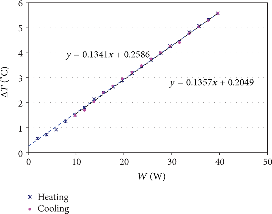
Schmidt-Milverton diagram for nanofluid (0.1%) at 25°C: The crosses represent the heating curve and the big points represent the cooling down curve.

Schmidt-Milverton diagram for nanofluid (0.1%) at 70°C: The crosses represent the heating curve and the big points represent the cooling down curve.
In such fluid considered as molecular mixtures, the processes of occurrence of instability involve also a mass transfer mechanism. This parameter will have an impact on how heat is transferred and can accelerate the threshold critical temperature gradient. This mass transfer contribution remains at this time a point requiring further investigations. It depends on the chemical natures of the dispersed nanoparticles, solvent, on composition, and on temperature
The slopes and the beginning of the convection depend also on the geometric parameters of the studied volume (the height and the surface of the discs).
For each set of experiments, the height and the surface of the working fluid are kept constant. The experimental conductive line slope in the Schmidt-Milverton diagram allows accurate measurement of thermal conductivity. From one side, the slope of the distilled water is used as reference and on the other side the slope of the desired solution gives its thermal conductivity.
The measured thermal conductivity is summarized in Table 1. Figure 5 represents its dependence on nanofluid concentration and on liquid temperature.
Experimental values of the thermal conductivity nanofluids based on NTC.

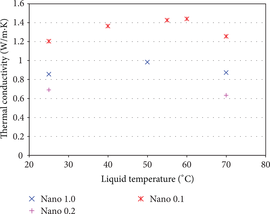
Temperature and concentration effect on measured thermal conductivity. The different symbols correspond to the different mass fractions of nanofluids shown in the insert.
4. Discussion
It can be seen that for the same liquid temperature, the thermal conductivity is rather higher for nanoparticles mass fraction of 0.1% than other concentrations. Also, for a given nanoparticles concentration (e.g., 0.1%), the thermal conductivity is a nonlinear function of the temperature.
It is obvious that those parameters affect the thermal conductivities values but the relationship for either thermal conductivity versus liquid temperature or versus particle concentration is nonlinear.
Our results confirm that the use of nanofluids as working fluid can enhance significantly its thermal performance but the dependency of this effect on nanoparticles concentration and temperature does not appear monotonous. There is a disagreement in the literature on this respect. As an example the results of Das et al. [9] confirm a strong temperature dependence on thermal conductivity of Al2O3 and CuO nanofluids. Prasher et al. [14] have reported a slight temperature dependence of CNT nanofluids thermal conductivity. On the other hand, Yang and Han [15] had experimentally found that Bi2Te3 nanorods in FC72 and in oil thermal conductivity decrease with temperature.
Most studies on nanofluids have reported that thermal conductivity linearly increases with particle concentrations [2, 6]. However there are also a few studies that indicate nonlinear behaviour [3, 4].
There are various possible sources of measurement uncertainties and the different experimental results cannot be strictly compared. The experimental measurement techniques and the nanofluids characteristics are very different. One possible reason of dispersion in the results is the existence of different aggregation states of nanoparticles and that can probably result from different preparation and handling techniques. The analysis of our experiment device at the end of the experiment shows some deposit on the discs that can be an important parameter in increasing or decreasing heat transfer. The used solution instead appears to be very stable for months, and in any case no deposit was observed in the bottle up to after the experiments.
At this moment we are not able to explain the origin of these discrepancies in published data of the nanofluid thermal conductivity.
In fact it will be interesting to complete the benchmark study of Buongiorno et al. [16] which does not include the carbon nanotubes solutions. Experimental results obtained could then be related to theoretical models as those described, for example, in Cherkasova and Shan [17, 18].
In this benchmark perspective, one should work with perfectly defined fluid and we propose our technique as one possible measurement technique.
5. Conclusions
Despite many experimental and theoretical studies [1, 19, 20] to understand the mechanism and thermal characteristic of nanofluids, the behavior of thermal proprieties of these nanofluids cannot be predicted and the science behind the thermal conductivity enhancement is still unclear. That is why very high attention is given on how experiment will be performed. The reliability of this work is to present a set-up and the associated experimental protocol to measure the thermal conductivity of nanofluids in a conductive regime with very good thermal control. To test the technique, single-walled carbon nanotubes dispersed in water by a two-step process were studied as function of temperature and composition. The experimental method has been found to be appropriate for prevention of natural convection and measurement seems correctly performed in the conductive regime. In any case, it was found that carbon nanotubes dispersed in water increase the thermal conductivity of the basic fluid. The dependence of thermal conductivity on nanoparticles concentration and the mean temperature of the liquid was tested and was found to be nonlinear.
The analysis of our experiment device at the end of the experiment shows some deposit on the discs. This effect will be discussed elsewhere in another paper.
In any case the reproducibility of results is outstanding and the set-up and protocol presented in this paper, including the use of a calibration fluid, provide excellent results for many other fluids too.
Footnotes
Acknowledgment
The authors gratefully acknowledge the Belgian Service of Science, Technics and Culture for supporting this research through The Belgian PRODEX program DCMIX.