Distributed k -Coverage Decision Scheme for System Deployment in Mobile Sensor Networks

Abstract

K-coverage sensor deployment is an important issue in wireless sensor networks (WSNs) applications. This is because an efficient topology structure significantly affects the quality of service and lifetime of WSNs. In the present work, we study the sensor deployment problem and propose novel distributed decision schemes to guide sensor movement to achieve k-coverage deployment. In our schemes, the kth order Voronoi diagram is used to discover the regions that do not meet the k-coverage requirement. Two different movement strategies are designed to determine the optimal location of each mobile sensor through local topological information. Finally, simulation results validate the effectiveness and accuracy of the proposed schemes.

1. Introduction

Such features as reliability, low cost, and ease of deployment make wireless sensor networks (WSNs) [1–3] convenient for monitoring hostile environments, including battlefields and disaster areas. In these applications, sensors are randomly dropped from aircrafts or other kinds of moving vehicles because manual interference is impossible. However, random deployment cannot guarantee that the sensors are evenly scattered in the monitored region. Additionally, when sensors run out of power, the coverage performance of a WSN worsens even further. Therefore, to improve fault tolerance and accuracy of data collection, we consider the k-coverage problem, where each point within the field can be monitored by at least k sensors.

Previous studies on k-coverage deployment can be broadly categorized into two types: centralized schemes and distributed schemes. The problem of centralized deployment has been tackled in previous literature [4–6]. Generally, using centralized deployment algorithms is easier for both stationary targets and moving targets with known and static movement patterns to achieve more precise deployment results. However, for an unknown and changing environment, centralized algorithms are not flexible enough to adapt to these changes. In [7, 8], the authors proposed various distributed schemes to address the k-coverage problem. These distributed algorithms feature self-organized sensors that carry out network tasks, thereby reducing messaging cost while improving the sensors' adaptability to dynamic conditions. However, it is assumed in these schemes that a sufficient number of sensors are provided. Therefore, a distributed k-coverage decision scheme for system deployment with limited sensors is still needed.

Most of the traditional support decision techniques [9–12] are all designed in a centralized manner and cannot be applied to a decentralized system. In this paper, we propose a novel distributed algorithm to minimize the number of deployed sensors while maximizing k-coverage sensing performance. In our algorithm, the kth order Voronoi diagram is adopted by dividing the entire region into subregions to detect coverage holes in each iteration. After determining the target region, our distributed algorithm calculates the optimal locations for sensors using local topological information only. Finally, we conduct various experiments to validate the performance of the proposed schemes.

The rest of this paper is organized as follows. In Section 2, we review previous work related to ours. The relevant description about the definition of k-coverage and then properties of the kth Voronoi diagram are introduced in Section 3. The k-coverage deployment scheme is presented in Section 4. We evaluate our algorithm in Section 5, followed by conclusions in Section 6.

2. Related Work

Most of the previous studies on the k-coverage problem focus on determining the optimal set of active sensors and assume that sensor network is densely deployed. Hefeeda and Bagheri [4] proposed a centralized approximation algorithm to obtain the minimum number of active sensors. Motivated by the divide-and-conquer concept, a randomly ordered activation and layering protocol (ROAL) has been discussed in [8]. ROAL builds k layers for the network in a distributed manner to guarantee k-coverage, where each layer can individually provide 1-coverage by selecting a disjoint subset of sensors without using location information. In the literature, static sensors are also assumed to be randomly deployed in the monitored region. Hence, a densely deployed network is constructed with the desired coverage level. However, redundancy is inevitably confronted.

The problem of mobile sensor k-coverage deployment has been studied in recent years. Wang and Tseng [7] developed a practical method, which aims at determining the minimum set of sensors and their locations. In order to move the sensors to the designated positions, they proposed a dispatch scheme that can minimize the energy consumption caused by sensor movement. A novel algorithm based on the nonuniform grid has been proposed by Sheu et al. in [5]. The authors designed a greedy deployment scheme to improve the k-coverage performance by placing new sensors in their precalculated locations in each iteration. However, mobile sensors are assumed to be static after they move to their designated locations. Therefore, sensors cannot dynamically adjust the network topology to maintain coverage performance in case of sensor malfunction or battery depletion.

The authors of a previous work [6] proposed a centralized algorithm that can determine uncovered positions by constructing the kth order Voronoi diagram of sensors. They designed a scheme to obtain the maximum subset of the relocatable sensors to repair the uncovered region. However, this scheme only moves the redundant sensors, which goes against the requirement of even deployment.

Compared with these previous studies, our work has two major contributions: (1) it addresses the problem of maximizing the k-coverage in a network with a certain number of mobile sensors and (2) we propose two novel schemes that move the sensors in an autonomous and distributed manner. In our schemes, a sensor only considers the local topological information and then conducts the movement in the local area.

3. Preliminaries

In this section, we introduce the network model, problem statement, and definitions that we use throughout this paper. Some notations are also listed in Table 1.

Table 1

Notations.

Notation	Description
$Ω$	The monitored region
$C (p, r)$	A circular region with center p and radius r
p	A point within the monitored region $Ω$
$r_{s}$	Sensing radius of sensor
$r_{c}$	Communicating radius of sensor
n	Number of the deployed sensors
S	The set of n sensors ${s_{1}, s_{2}, \dots, s_{n}}$
$d (., .)$	Euclidean distance between two 2D points
H	A subset of S
$V (s_{i})$	The Voronoi region of sensor i
$Vor (S)$	The 1th order Voronoi diagram
$V_{k} (H)$	The kth order Voronoi region of H
q	The kth farthest point of $V_{k} (H)$
${Vor}_{k} (S)$	The kth order Voronoi diagram

3.1. Network Model

Consider that n sensors with uniform sensing and communication radius are randomly deployed in region Ω, which is convex and obstacle-free. The coverage and communication of sensors are defined by both 0-1 binary models. Sensors are also aware of their locations, which can be obtained using some localization techniques, such as range-based and range-free location schemes [13, 14].

In this paper, we focus on maximizing k-coverage deployment, which can be divided into two steps, namely, k-coverage detection and k-coverage redeployment. The former aims to detect the coverage holes that are not covered at any point by at least k sensors, while the latter aims to determine the optimal locations for mobile sensors such that k-coverage deployment can be achieved.

3.2. Definitions

Definition 1 (1-coverage).

If each point p within Ω can be monitored by at least one sensor, this is called 1-coverage. In other words, the shortest Euclidean distance between point p and any sensor is no more than sensing radius $r_{s}$ . Thus, the above description [15] can be formulated as follows:

\begin{matrix} \min (d (s, p)) \leq r_{s}, \forall p \in Ω, s \in S . \end{matrix}

(1)

Definition 2 (k-coverage).

If each point p within Ω can be monitored by at least k sensors, this is called k-coverage. Similarly, the above description can be formulated as [4]

\begin{matrix} d (s_{i}, p) \leq r_{s}, \forall p \in Ω, s_{i} \in H, H \subset S, | H | \geq k . \end{matrix}

(2)

Definition 3 (Voronoi polygon).

The Voronoi polygon $V (s_{i})$ is defined as the set of points that are closer to $s_{i}$ than to any other sensors. Clearly,

\begin{matrix} V (s_{i}) = {p | s_{i} \in S, \forall s_{j} \in S, j \neq i, d (p, s_{i}) \leq d (p, s_{j})} . \end{matrix}

(3)

Definition 4 (kth order Voronoi polygon).

The kth order Voronoi polygon $V_{k} (H)$ is defined as the set of points having a subset H of k sensors in S as its k nearest neighbors [16] given as

\begin{matrix} V_{k} (H) = {p | \forall s_{i} \in H, \forall s_{j} \in S - H, d (p, s_{i}) < d (p, s_{j})} . \end{matrix}

(4)

Definition 5 (kth farthest point of $V_{k} (H)$ ).

Suppose $F (x, H)$ is the longest distance between point x and any point within set H, for a point q from set $V_{k} (H)$ ; if the value of $F (q, H)$ is higher than that of any other point x in $V_{k} (H)$ , q is the kth farthest point of $V_{k} (H)$ [6] given as

\begin{matrix} F (x, H) = \max (d (x, s_{i})), \forall s_{i} \in H, H \subset S, | H | = k, \\ F (q, H) = \max (F (p, H)), \forall p \in V_{k} (H) . \end{matrix}

(5)

Definition 6 (Voronoi diagram).

The Voronoi diagram is a kind of decomposition of a given 2D space, consisting of a series of Voronoi polygons. Figure 1 shows two examples of the Voronoi diagram. These are given by

\begin{matrix} Vor (S) = \cup V (s_{i}), s_{i} \in S, \\ Vo r_{k} (S) = \cup V_{k} (H), H \subset S, | H | = k . \end{matrix}

(6)

Figure 1

Voronoi diagrams.

4. Algorithm

In this section, we use the properties of the kth order Voronoi diagram to solve the coverage detection problem raised in Section 3. We also propose two different distributed self-deployment approaches to obtain the optimal locations for mobile sensors.

4.1. k-Coverage Detection

Most previous studies on the 1-coverage problem use the Voronoi diagram to detect a coverage hole and estimate its size [17, 18]. According to the property of the Voronoi diagram, each point within a Voronoi polygon is the closest to just one Voronoi site that lies within this polygon, as shown in Figure 1(a). Therefore, if the sensing disk of a sensor cannot cover its Voronoi polygon, a coverage hole exists in this polygon. As can be seen from Figures 1(a) and 1(b), the number of 2nd order Voronoi polygons is larger. Moreover, the number of polygons increases while the coverage degree increases. Second, in a higher coverage degree situation, it is hard to find the target sensors corresponding to the polygon and to check whether the sensing disks of sensors can cover the polygons. Due to the complexity of the k-coverage problem, it is difficult to accurately calculate the size of a coverage hole in Ω using the kth order Voronoi diagram; it is also difficult to detect all the coverage holes accurately. Definition 2 provides an approximate way to solve this problem. If the region Ω is k-covered, an arbitrary point within Ω is covered by at least k sensors. In other words, if there is a subset of points in Ω that cannot satisfy k-coverage requirement, the entire region Ω is thereby not k-covered. Moreover, it has been proved that the possibility of the farthest points that are not k-covered is higher than that of any other point, and the kth farthest points of the kth order Voronoi polygons are in the vertices set of these polygons [6]. Therefore, we select a particular point set that consists of vertices of all kth order Voronoi polygons and boundary intersections in order to check the coverage degree of each point within it. If any uncovered point exists, sensors decide the optimal locations to move in the k-coverage redeployment phase; otherwise, they evaluate the coverage rate. However, although the vertices of all Voronoi polygons are k-covered, some points within the polygons may still not be k-covered. Therefore, we propose an approach based on grid to evaluate the coverage rate, which is defined as the percentage of the grid monitored by at least k sensors [19].

In the coverage detection stage, each sensor first broadcasts its location and receives information from its neighbor sensors, based on which its local kth order Voronoi diagram can be constructed. In order to detect the uncovered point, the sensor calculates the coverage degree of each vertex of the kth order Voronoi polygons and the boundary intersection points, which is equal to the number of sensors that cover the referred point. The points with coverage degrees lower than k are selected to constitute the uncovered point set U.

In some cases, the local kth order Voronoi polygons of the sensors are well covered, since the local sensor density is high in initial deployment, resulting in the immobility of sensors located inside the clusters. However, there are still some subregions that cannot meet the coverage requirement. To deal with this problem, we propose a preprocessing scheme that only runs in the first round to scatter the sensors. To begin with, each sensor checks whether it is redundant. If a sensor is a redundant one, its uncovered point set is null. These uncovered points located in the sensor's sensing disk are k-covered. Thus, it will conduct a randomized process to select a random position within the monitor region as its destination.

4.2. k-Coverage Redeployment

For the following phase, we design two k-coverage redeployment algorithms to move sensors from the dense region to spare region to maximize the sensing coverage.

We design specific rules to guide the movement of the sensors. First, without decreasing the k-coverage rate of a currently monitored region, movements of the relocatable sensors are supposed to be toward an uncovered area. Second, when determining the target location, each sensor should avoid increasing the sensor density of the local area because of its movement. Considering these rules, movement strategies are proposed to address the k-coverage redeployment problem.

4.2.1. The Minimum Covered Circle Based Algorithm (MCCA)

Based on the concept of the smallest enclosing disk, we propose a novel distributed deployment algorithm that guides sensors to move closer toward uncovered points. This is called the minimum covered circle based algorithm (MCCA) and can determine the optimal location if the uncovered point is detected (see Algorithm 2). This location is at the center of the smallest circle, which can cover both uncovered points and those within the sensing disk of the sensor that are not k-covered. The distributed algorithm has four main steps described below. (1)

Determine the target uncovered point of sensor $s_{i}$ to be repaired. In this step, the target uncovered point of sensor $s_{i}$ is obtained by comparing distances between sensor $s_{i}$ and each point within the point set U. Then, sensor $s_{i}$ selects the point outside its sensing area with the shortest distance as its target uncovered point.

(2)

Generate the point set M. Once sensor $s_{i}$ determines its target point, the next step is to generate the point set M. Given a point set that consists of vertices of the kth order Voronoi polygons and the boundary intersection points, only the point that is located in the sensing disk of the sensor and simultaneously monitored by at most k sensors is added to set M. Moreover, the target point is included in set M.

(3)

Calculate the optimal position for sensor $s_{i}$ . The third step is the core part of our algorithm. Here, sensor $s_{i}$ calculates the minimum circle that can cover all points within the point set M (see Algorithm 1). If the radius of the circle is less than the sensing radius, the optimal location of sensor $s_{i}$ is the center of this circle. Otherwise, the algorithm calculates the minimum circle of the new point set $M^{'}$ , which excludes the target point from set M. Similarly, if the distance between the center of the new circle and each point within point set $M^{'}$ is smaller than the sensing range, sensor $s_{i}$ moves to the center of the new circle. In particular, the point set $M^{'}$ contains one point; the optimal location is on the straight line connecting the point and target point, whose distance to the point is equal to the sensing range. In addition, for a free sensor whose sensing disk can be monitored by at least k sensors except this sensor, it moves toward its target point and stops at a distance of its sensing radius to it.

(4)

Check the optimal location. Once the optimal location of sensor $s_{i}$ is determined, another critical issue is to check whether another sensor already exists there or if its local density is higher than the desired density. If the high-degree clustering occurs, an available solution to this problem is to replace the optimal location with the midpoint between the current sensor location and the optimal location.

Algorithm 1: Calculate the minimum circle $C (O, R)$ ; input: $M = {p_{1}, p_{2}, \dots, p_{n}}$ ; output: $O, R$ .

(1) for $i = 1$ to $n - 1$

(2) for $j = i + 1$ to n

(3) calculate the circle $C (p_{i}, p_{j}), o = (p_{i} + p_{j}) / 2, r = d (p_{i}, p_{j}) / 2$ ;

(4) if $d (p_{u}, o) \leq r$ , where $\forall p_{u} \in M$ then

(5) record it;

(6) choose one with minimum radius and assign the value to $C (O, R)$ ;

(7) if find the $C (O, R)$

(8) return

(9) else

(10) for $i = 1$ to $n - 2$

(11) for $j = i + 1$ to $n - 1$

(12) for $k = j + 1$ to n

(13) calculate the circumcircle $C (p_{i}, p_{j}, p_{k})$

(14) if $p_{v}$ in $C (p_{i}, p_{j}, p_{k})$ , where $\forall p_{v} \in M$ then

(15) record it; and

(16) Choose one with minimum radius and assign the value to $C (O, R)$ .

Algorithm 2: The minimum covered circle based algorithm (MCCA); input: $s_{i}, U, N, k$ ; output: $s_{i}$ .

(1) Generate the moving target point v;

(2) Generate the point set M;

(3) if $n \geq 2$ (the size of the point set M)

(4) calculate the minimum circle $C (O, R)$

(5) $s_{i} = O$

(6) else

(7) $d (v, p_{m}) = r_{s}$ , $p_{m}$ is on the line $v s_{i}$

(8) $s_{i} = p_{m}$

(9) Check the target location and determine the final location.

4.2.2. The Geometric Center-Based Algorithm (GCA)

Similar to MCCA, the geometric center-based algorithm (GCA) is another form of the movement strategy; it determines the optimal location by calculating the geometric center of the convex hull of the point set. The algorithm (Algorithm 3) also has four main steps as listed below. (1)

Determine the target point of sensor $s_{i}$ to be repaired following the same procedure as that used in the MCCA.

(2)

Generate the point set M. This is also the same as that used in the MCCA.

(3)

Calculate the optimal positions of sensors. After collecting the local topological information, sensors $s_{i}$ decide their optimal movement locations. In this process, they first calculate the convex hull of the point set M, which is the minimum polygon containing all the points within point set M. After the convex hull with n (a given parameter) sides has been calculated, it is divided into $n - 2$ triangles, after which the area and the center of gravity of these triangles are calculated. According to the weighted average method, the geometric center of the convex hull can be calculated and can serve as the optimal location. If the size of the set M is smaller than three, the optimal location in this algorithm is considered the same as shown in MCCA.

(4)

Check the optimal location. This is also the same as that used in the MCCA.

Algorithm 3: Calculate the geometric center; input: $M = {p_{1}, p_{2}, \dots, p_{n}}$ ; output: O.

(1) Calculate the convex hull of the set $M, C H (M) = {p_{1}, p_{2}, \dots, p_{m}}$ and sort the points in

anti-clock order;

(2) Divide the convex hull with m sides into $m - 2$ triangles;

(3) Calculate the area and the center of gravity of these triangles

$S = {s_{1}, s_{2}, \dots, s_{m - 2}}, G = {g_{1}, g_{2}, \dots, g_{m - 2}}$ ;

(4) Calculate the center of gravity of the convex hull ${\bar{G}}_{x} = \sum_{i = 1}^{m - 2} s_{i} \cdot {g_{i}}_{x} / \sum_{i = 1}^{m - 2} s_{i}$ ,

${\bar{G}}_{y} = \sum_{i = 1}^{m - 2} s_{i} \cdot {g_{i}}_{y} / \sum_{i = 1}^{m - 2} s_{i}$ , assign the value to O.

5. Performance Evaluation

In this section, we chose the sensor coverage rate and the average moving distance as performance metrics in order to validate the previous analysis of the proposed algorithms. Coverage is a significant measurement used to evaluate the quality of a WSN. Furthermore, the objective of the sensor deployment scheme is to maximize the sensing coverage and minimize the number of sensors while maintaining a certain degree of sensing coverage. The cost of constructing a WSN contains the sensor cost and the energy consumption. During the deployment stage, sensor networks usually consume a large amount of energy due to the movements of mobile sensors. Thus, we also consider the average moving distance to validate the performance of our deployment schemes.

The performance evaluation parameters we consider include sensor density and coverage level. In the experiments, we randomly deploy different numbers of sensors in the monitored area under two coverage levels. Moreover, we also consider various field sizes to validate the availability of our algorithm. Without loss of generality, we execute our schemes under two different sensor deployment scenarios, namely, normal deployment and uneven deployment.

The region size is 100 m * 100 m, and the sensing radius and communication radius are 10 m and 20 m, respectively.

5.1. Coverage

We randomly deploy different numbers of sensors in the monitored region under the two coverage levels. The initial coverage of the sensor networks is shown in Figure 2. Compared with static sensor deployment, our distributed self-deployment algorithms can deploy less mobile sensors while achieving the same coverage requirement. In Figure 3(a), the initial coverage of the target area with 90 randomly deployed sensors is 73%, while the target area can reach 91% coverage using our algorithms. To reach the same coverage, about 155 static sensors are needed.

Figure 2

Coverage rate under different k-covered requirements.

Figure 3

Coverage rate under the 2-coverage level.

5.1.1. 2-Coverage Level

In this section, we randomly deploy 4 different numbers of sensors ranging from 90 to 120, in increments of 10 sensors under a coverage level $k = 2$ scenario. We compare our distributed algorithms against the Shen and Wu algorithm [6]. Simulation results are shown in Figures 3 and 4.

Figure 4

Moving distance under the 2-coverage level.

As can be seen from Figures 3(a) and 3(b), both MCCA and GCA perform better compared with the Shen and Wu algorithm under random deployment. This is because the Shen and Wu algorithm, which repairs the uncovered region by moving only the redundant sensors, can only evenly distribute a small number of redundant sensors. In addition, our algorithms exhibit similar performance under higher sensor densities, because the number of deployed sensors is close to the minimum number of sensors required in the monitored region.

In Figures 4(a) and 4(b), we can see that the average moving distance after ten rounds in the Shen and Wu algorithm gradually increases with the increase of sensor number. This is because the percentage of relocatable sensors increases under higher sensor density. In comparison, in our algorithms, the average moving distance under high density deployment is smaller than that of low density deployment. In addition, the average moving distance by GCA is mostly smaller than that of MCCA, because the geometric center calculated by GCA is always located inside the convex hull.

5.1.2. 3-Coverage Level

To evaluate the performance of our algorithms under the 3-coverage level, we consider the monitored region to be a 100 m * 100 m field. Motivated by k-layer coverage [8], we distribute 135, 150, 165, and 180 sensors in the monitored regions. The results are shown in Figures 5 and 6.

Figure 5

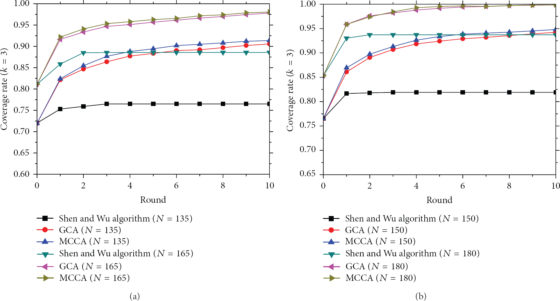
Coverage rate under the 3-coverage level.

Figure 6

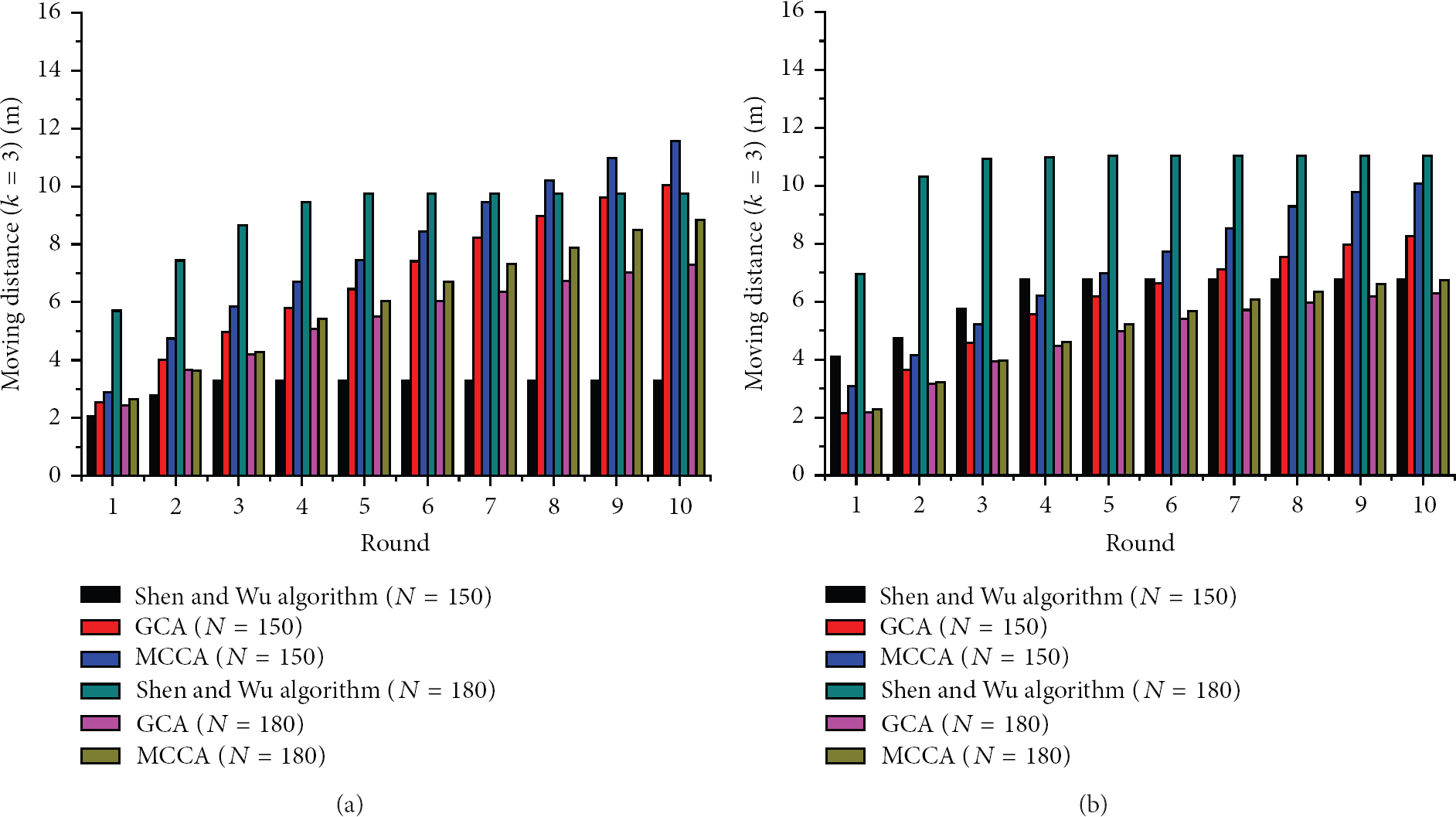
Moving distance under the 3-coverage level.

Figures 5(a) and 5(b) represent a comparison for the coverage rates among the Shen and Wu algorithm and the GCA and MCCA under different node densities. We can see that our distributed algorithms provide better coverage than the Shen and Wu algorithm even in the deployment scenario. This is expected because our algorithms can fully utilize each mobile sensor in the network to maintain the uncovered region using local topological information.

As indicated in Figures 6(a) and 6(b), the Shen and Wu algorithm has much higher average moving distance under high sensor density; this is because more mobile sensors can move from the dense region to the spare region when the sensor density increases. In contrast, the moving distance in both GCA and MCCA declines with an increase in the amount of deployed sensors. This is mainly due to the fact that some sensors can decide their final locations at the initial stage under high density deployment.

5.2. Field Size

To demonstrate the validity of our distributed algorithm in terms of feasibility in a large-scale network, we varied the scale of the target field from 100 m * 100 m to 300 m * 300 m and considered the scenario in which 115 sensors are randomly deployed into each 100 m * 100 m subregion; each point within the area is monitored by at least 2 sensors. The results of different algorithms after ten rounds are shown in Table 2.

Table 2

Different scales of the target field.

Algorithms	Coverage degree	Scale of region	Coverage rate	Moving distance (m)
MCCA	$k = 2$	100 m * 100 m	98.85%	7.25
		200 m * 200 m	99.04%	7.16
		300 m * 300 m	99.47%	7.01
GCA	$k = 2$	100 m * 100 m	98.43%	6.84
		200 m * 200 m	98.66%	6.72
		300 m * 300 m	99.12%	6.55

From Table 2, we can see that the scale of the network has little effect on the performance of our algorithms, because the sensors only communicate with their neighbor sensors and the movements are conducted within the local area. We also notice that the coverage rate shows an ascending trend with the increasing of the network scale. This is because the sensors near the boundary of the subregion have sensing disks that also largely cover what is outside the boundary. Thus, enlarging the network scale can decrease the ratio of sensors near the boundary.

5.3. Deployment

The simulation results in the previous sections demonstrate the availability and effectiveness of our algorithms in normal deployment. In this section, we measure the performance in an uneven deployment scenario, where 120 sensors are randomly distributed in the bottom left quarter area (50 m * 50 m) in region Ω. The coverage rate and average moving distance under different rounds are shown in Figure 7.

Figure 7

Uneven deployment.

Figure 7 indicates that our algorithms can deal efficiently with high-degree clustering in an uneven deployment scenario. The randomized process in the first round facilitates the even deployment of the clustered sensors throughout the entire region. In addition, we notice that in the Shen and Wu algorithm [6] the curve of the coverage is an S-shaped growth curve. This is because the increase in coverage is determined by the number of both the relocation positions and the relocatable sensors. Moreover, in light of the high-degree clustering, the number of relocation positions determined by the kth order Voronoi diagram is far less than that of the relocatable sensors in the first round. After several rounds, the number of relocatable sensors gradually decreases since the distribution of the sensors becomes more even.

6. Conclusion

In this paper, we studied the problem of k-coverage deployment in mobile WSNs. Based on the kth order Voronoi diagram, the target region which is not k-covered under random deployment was detected. We then proposed two distributed self-deployment algorithms to maximize sensing coverage. In simulations, the results validate the performance of the proposed schemes and demonstrate their effectiveness and availability.

In our network model, we assume that coverage and communication of the sensors use the binary model. However, the probabilistic sensing model of the sensors is more practical, thus deserving further study. Also, heterogeneous WSNs and hybrid networks, where both static and mobile sensors are distributed, are also worthy of further study.

Footnotes

Conflict of Interests

The authors declare that there is no conflict of interests regarding the publication of this paper.

Acknowledgments

This research is partially supported by research grants from the National Science Foundation of China under Grant nos. 71271148 and 71071105, a National Science Fund for Distinguished Young Scholars of China under Grant no. 70925005, and the Program for Changjiang Scholars and Innovative Research Team in the university (IRT1028).

References

Yang

Sun

Y. G.

Taheri

Zomaya

A. Y.

DLS: a dynamic local stitching mechanism to rectify transmitting path fragments in wireless sensor networks

Journal of Network and Computer Applications 2013 36 1 306 315

10.1016/j.jnca.2012.05.012

Cao

Chen

Zhang

Sun

Development of an integrated wireless sensor network micro-environmental monitoring system

ISA Transactions 2008 47 3 247 255

2-s2.0-44449132515

10.1016/j.isatra.2008.02.001

Zhou

Wang

Lian

Zhang

Vasilakos

A. V.

Jing

Availability-aware multimedia scheduling in heterogeneous wireless networks

IEEE Transactions on Vehicular Technology 2011 60 3 1161 1170

2-s2.0-79952854696

10.1109/TVT.2011.2104420

Hefeeda

Bagheri

Randomized k-coverage algorithms for dense sensor networks

Proceedings of the 26th IEEE International Conference on Computer Communications (INFOCOM '07)

May 2007

Anchorage, Alaska, USA

2376 2380

2-s2.0-34548297823

10.1109/INFCOM.2007.284

Sheu

J.-P.

Chang

G.-Y.

Chen

Y.-T.

A novel approach for κ-coverage rate evaluation and re-deployment in wireless sensor networks

Proceedings of the IEEE Global Telecommunications Conference (GLOBECOM '08)

December 2008

New Orleans, Louisiana

341 345

2-s2.0-67249112699

10.1109/GLOCOM.2008.ECP.73

Shen

Minimum sensor relocation for κ-coverage in wireless sensor networks

Proceedings of the International Conference on Communications and Mobile Computing (CMC '10)

April 2010

Shenzhen, China

CPS

274 278

2-s2.0-77953994017

10.1109/CMC.2010.251

Wang

Y.-C.

Tseng

Y.-C.

Distributed deployment schemes for mobile wireless sensor networks to ensure multilevel coverage

IEEE Transactions on Parallel and Distributed Systems 2008 19 9 1280 1294

2-s2.0-49349106443

10.1109/TPDS.2007.70808

Kim

E. J.

Yum

K. H.

ROAL: a randomly ordered activation and layering protocol for ensuring K-coverage in wireless sensor networks

Journal of Networks 2008 3 1 43 52

2-s2.0-78651525407

Peng

Kou

Shi

Chen

A descriptive framework for the field of data mining and knowledge discovery

International Journal of Information Technology and Decision Making 2008 7 4 639 682

2-s2.0-58149235001

10.1142/S0219622008003204

10.

Peng

Zhang

Tang

An incident information management framework based on data integration, data mining, and multi-criteria decision making

Decision Support Systems 2011 51 2 316 327

2-s2.0-79953753719

10.1016/j.dss.2010.11.025

11.

Kou

Peng

Chen

Shi

Multiple criteria mathematical programming for multi-class classification and application in network intrusion detection

Information Sciences 2009 179 4 371 381

2-s2.0-56949107719

10.1016/j.ins.2008.10.025

12.

J. W.

Song

Y. L.

Community detection in complex networks using extended compact genetic algorithm

Soft Computing 2013 17 6 925 937

10.1007/s00500-012-0942-1

13.

Savvides

Han

C.-C.

Strivastava

M. B.

Dynamic fine-grained localization in ad-hoc networks of sensors

Proceedings of the 7th Annual International Conference on Mobile Computing and Networking

July 2001

Rome, Italy

ACM

166 179

2-s2.0-0034775930

14.

Bulusu

Heidemann

Estrin

GPS-less low-cost outdoor localization for very small devices

IEEE Personal Communications 2000 7 5 28 34

2-s2.0-0034291601

10.1109/98.878533

15.

J.-S.

Kao

H.-C.

Distributed K-coverage self-location estimation scheme based on Voronoi diagram

IET Communications 2010 4 2 167 177

2-s2.0-75649096049

10.1049/iet-com.2009.0288

16.

Lee

D. T.

On k-Nearest Neighbor Voronoi Diagrams in the Plane

IEEE Transactions on Computers 1982 31 6 478 487

2-s2.0-0020141081

17.

Ghosh

Estimating coverage holes and enhancing coverage in mixed sensor networks

Proceedings of the 29th Annual IEEE International Conference on Local Computer Networks (LCN '04)

November 2004

68 76

2-s2.0-20544442644

10.1109/LCN.2004.53

18.

Wang

Cao

Berman

La Porta

T. F.

Bidding protocols for deploying mobile sensors

IEEE Transactions on Mobile Computing 2007 6 5 515 528

2-s2.0-33947622591

10.1109/TMC.2007.1022

19.

Jin

J.-Y.

Wang

Kim

Yang

ECCRA: An energy-efficient coverage and connectivity preserving routing algorithm under border effects in wireless sensor networks

Computer Communications 2008 31 10 2398 2407

2-s2.0-44549084151

10.1016/j.comcom.2008.03.001

Distributed k -Coverage Decision Scheme for System Deployment in Mobile Sensor Networks

Abstract

1. Introduction

2. Related Work

3. Preliminaries

3.1. Network Model

3.2. Definitions

Definition 1 (1-coverage).

Definition 2 (k-coverage).

Definition 3 (Voronoi polygon).

Definition 4 (kth order Voronoi polygon).

Definition 5 (kth farthest point of V k ( H ) ).

Definition 6 (Voronoi diagram).

4. Algorithm

4.1. k-Coverage Detection

4.2. k-Coverage Redeployment

4.2.1. The Minimum Covered Circle Based Algorithm (MCCA)

Algorithm 1: Calculate the minimum circle C ( O , R ) ; input: M = { p 1 , p 2 , … , p n } ; output: O , R .

Algorithm 2: The minimum covered circle based algorithm (MCCA); input: s i , U , N , k ; output: s i .

4.2.2. The Geometric Center-Based Algorithm (GCA)

Algorithm 3: Calculate the geometric center; input: M = { p 1 , p 2 , … , p n } ; output: O.

5. Performance Evaluation

5.1. Coverage

5.1.1. 2-Coverage Level

5.1.2. 3-Coverage Level

5.2. Field Size

5.3. Deployment

6. Conclusion

Footnotes

Conflict of Interests

Acknowledgments

References

Definition 5 (kth farthest point of $V_{k} (H)$ ).

Algorithm 1: Calculate the minimum circle $C (O, R)$ ; input: $M = {p_{1}, p_{2}, \dots, p_{n}}$ ; output: $O, R$ .

Algorithm 2: The minimum covered circle based algorithm (MCCA); input: $s_{i}, U, N, k$ ; output: $s_{i}$ .

Algorithm 3: Calculate the geometric center; input: $M = {p_{1}, p_{2}, \dots, p_{n}}$ ; output: O.