Wireless sensor networks (WSNs) consist of thousands of nodes that need to communicate with each other. However, it is possible that some nodes are isolated from other nodes due to limited communication range. This paper focuses on the influence of communication range on the probability that all nodes are connected under two conditions, respectively: (1) all nodes have the same communication range, and (2) communication range of each node is a random variable. In the former case, this work proves that, for , if the probability of the network being connected is , by means of increasing communication range by constant , the probability of network being connected is at least . Explicit function is given. It turns out that, once the network is connected, it also makes the WSNs resilient against nodes failure. In the latter case, this paper proposes that the network connection probability is modeled as Cox process. The change of network connection probability with respect to distribution parameters and resilience performance is presented. Finally, a method to decide the distribution parameters of node communication range in order to satisfy a given network connection probability is developed.
1. Introduction
Wireless sensor networks (WSNs) [1, 2] are a promising technology nowadays. The use of WSNs in numerous applications, such as forest monitoring, disaster management, space exploration, factory automation, secure installation, border protection, and battlefield surveillance, is emerging. WSNs technology is the basis of future network “Internet of Things” (IoT) [3], which offers a vision where anyone can interact with any addressable nodes (things or objects)—such as RFID tags, sensors, and mobile phones—anywhere and anytime. “Anywhere” suggests that any object is reachable from any location. From the network topology point of view, every node in WSNs should be able to, directly or through limited number of intermediate nodes, connect to any other nodes. This kind of network is called “connected network.” If the network is still connected after removing at most nodes, it is called k-connected network, where . A k-connected network guarantees that at least k different paths are available for transmitting signals from one node to any other nodes.
However, k-connected network is not always possible. In WSNs, sensor nodes are usually deployed in the areas of interest either randomly or according to a predefined distribution. In this case, it is likely that some nodes are isolated from other nodes. Therefore, the network connection is characterized by probability. On the other hand, the resilient problem, which indicates fault-tolerance capability in the presence of node failure, is also important in the probabilistic network. Our concern in this paper is the probability that the WSNs are a connected network and network resilience against the node failures.
Most of earlier studies focus on the model where each node in a network is the same and, for example, has the same communication range. However, WSNs nodes are usually heterogeneous. The communication range of the WSNs node may vary from one node to another, and even communication range of the same node may change over time. For instance, in a wireless network, the transmission power required for a node to reach another node is proportional to , where R is the transmission radius and α is the loss constant depending on the wireless medium of which typical value is between 2 and 4 and may vary from devices to devices [4]. According to various wireless communication technologies, communication range may vary from tens to thousands meters, such as IEEE 802.11 (25–600 m), Bluetooth (10–100 m), ZigBee (10–75 m), HomeRF (50 m), UWB (10 m), and WiMAX (1–50 km). Depending on how long nodes work, residual energy of battery powered devices decreases over time, so a node may try to shorten communication range in order to save energy. Environments where nodes are deployed, for example, indoor or outdoor, with or without obstacle, result in communication range quite different due to the interference, shadowing, fading, and pass loss [5].
This work concentrates on WSNs connection probability for both heterogenous and homogenous networks in terms of communication range. Assuming WSNs nodes are randomly and uniformly distributed, two problems are addressed in this paper: given a network where all nodes have the same communication range, how does the connection probability change as communication range increases? In the case that communication range is a random variable, what is the network connection probability?
Through analysis, this work finds that for and the number of nodes in the network is big enough and if the original network connection probability is, through increasing the communication range by constant, the probability of a network being connected increases from to . Explicit function is given in this paper. It turns out that, when a network is connected, it is also almost sure -connected(where n is the total number of nodes deployed andis a constant greater than 1), which is important for the WSNs resilient against the node failure. Afterwards, the connection probability problem with random communication range, which is often the real case in the WSNs, is studied. The model is reformulated as Cox process, and the connection probability is analyzed by simulation. A method for determining the distribution function parameters for a given connection probability is developed.
Our main contributions are as follows: first, this paper employs an effective and novel approach to obtain analytical results for homogenous WSNs connectivity, some of which have been validated by previous studies; second, we propose that the Cox process can be used to model heterogenous WSNs and the simulations are performed to reveal the relations between the network connection probability and its distribution parameters.
The rest of this paper is organized as follows. Section 2 introduces the basic concepts of network model and the problem to be addressed. In Section 3, derivation and verification in case that the network nodes have the same communication range are presented. In Section 4, communication range is modeled as a random variable. A brief introduction of related works is provided in Section 5 while Section 6 concludes our work.
2. Network Model and Problem Statement
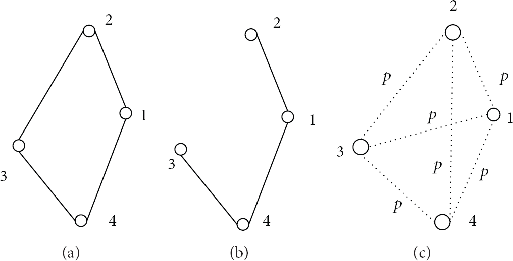
Usually, there are three methods to create links between nodes, as presented in Figure 1. One is k-nearest neighbor model. In this model, the network is formed by each node connecting to k-nearest neighbors; for example, in Figure 1(a), each node has 2 neighbors. The second is disc model. Node is modeled as a disk with communication radius r. The node s is linked to node u if the Euclidean distance between s and u is less than r; for example, in Figure 1(b), node 3 cannot connect to node 2 and node 1 because they are out of communication range of node 3. The last one is Erdös-Rényi random graph that connects any two nodes by the same probability which is inappropriate in the WSNs; for example, in Figure 1(c), each node connects other nodes with the same probability P. The k-nearest neighbor model can be achieved by changing communication range of each node until the number of neighbors reaches k. Disc model, on the other hand, connects those nodes that fall into its communication range. k-nearest neighbor model and disc model are different. k-nearest neighbor model makes sure that there is no isolated node, but disc model is characterized by the probability that a network does not have isolated nodes. Disc model is more plausible in the WSNs in the case that obtaining k neighbors is not always feasible. For instance, in wireless environment, some nodes may be unable to connect to a required number of neighbors due to the communication range limitation.
Different methods to connect nodes: (a) node connects 2 nearest neighbors; (b) node connects other nodes within its communication range; (c) node connects other nodes with same probability P.
The notations and basic network definitions that will be used throughout the paper are now introduced. Additional terminologies are referred to [6]:
n: total number of nodes deployed in target field, and ,
A: area of node deployed,
ρ: node density, defined as ,
t: expected number of neighbors of node.
Note that in this paper “log” means the logarithm to nature base e. Next, main definitions are introduced.
Definition 1.
Node's communication range is defined as the area where other nodes can receive its signal.
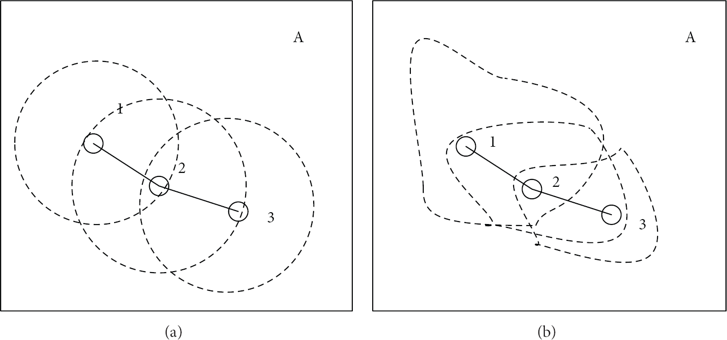
For a disk, the communication range is the circle with radius r. However, communication range is not necessary modeled as a disk. The communication range of radio is highly probabilistic and irregular [7, 8]. Figures 2(a) and 2(b) illustrate the ideal disk communication and irregular communication model, respectively. More importantly, the communication range of each node may not be the same. Note that the analysis in this section is a disk, but it can also apply to the irregular communication model.
(a) Disk communication model and (b) irregular communication model.
Definition 2.
denotes a network following disc model. More specifically, the network is formed by n nodes randomly and uniformly deployed in area A. The node is modeled as a disk with radius r.
This paper focuses on the probability of network being k-connected. A k-connected network implies that there are still alternative path(s) if one path failed, therefore a higher k indicates that the network is more resilient against failures. In this paper, k is used to evaluate the WSNs resilience. This property depends on many factors, such as communication range, node density ρ, node processing capability, node energy, and deployment environment. This paper is only interested in the impact of communication range on the connection probability. The problem can be stated as follows.
“Given WSNs with fixed node density ρ, in the cases in which node communication range is the same and different, how network connection probability and resilience performance change as node communication ranges vary?”
3. Homogenous Node Deployment in WSNs
This section considers that, in the network , each node has the same communication range. First, the mathematical model that will be used is presented. Based on this model, theoretical results are proved and validated by an example and simulations. In Section 4, the situation where communication range of each node is a random variable will be discussed.
3.1. Network Connection Probability Analysis
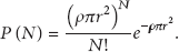
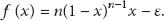
For uniformly distributed nodes with density ρ, the number of nodes in the area has a Poisson distribution [9]; therefore the probability of a node having N neighbor nodes is
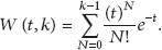
Number of node neighbor is also called the node's degree. The minimal degree of all nodes is called the network degree. If the network has n nodes, the probability of network is k-connected given by following well-known formula [9]:
Let
Note that t indicates the communication range of a node, but, if , t actually is the expected number of neighbors a node has.
Without loss of generality, assume that . For a real network the density of node indicates that the average number of nodes in unit area is one. However, whetheris equal to 1 is irrelevant in this model, because if ρ is not 1, say , then letting the results will be the same. In order to simplify denotation, define
The function can be written as when . In this section, the properties of are analyzed, namely, -connected network. Two points are found out where almost starts and stops growing in order to show that the connection probability increases from near to reach .
Proposition 3.
Letting and , then following statements hold:
for every, there existssuch that;
has a flex point at.
Proof.
(1) First, (5) is a monotonically increasing function for any (note that is the Taylor expansion of, and ); see Figure 3(a).
Now consider the first and second derivative functions of :
It is evident that vanishes at and . Furthermore, for and for . Therefore, is an increasing function in the interval and a decreasing function in . Hence, reaches the maximum value at (see Figure 3(a)). On the other hand, since , by applying Bolzano Theorem, for every , there exists , such that (Figure 3(b)).
(2) It is derived from the proof of statement above.
Network connection probability function and corresponding and (a); values and for a given ɛ and (b).
The proof of the previous proposition can be applied to obtain the following result.
Theorem 5.
Let , , , and . Then there exists a constant number of neighbors, , for which the network becomes connected with probability increasing from to .
Proof.
First, it can be observed that satisfies the hypothesis in Proposition 3 (1) since ; therefore . Let and define as
Then, the goal is to find the roots of (8). For this purpose, consider the derivative function:
Note that is the function under the change of variable , and by applying the proof of Proposition 3 there exist only two roots and of in the interval . Newton method can be used to find out the approximation of roots and . However, its accuracy depends on the initial value, which should be close enough to the real root. Letting be the initial value, according to (8) and (9), yields
Additionally, the inequality holds from the proof of Proposition 3; then Newton method can be applied. Let as the initial value to approximate and (where ) as the initial value to find :
Taking into account that we have when and , therefore
Note that . Letting , , and defining , according to (12), we obtain
Finally, taking into account that , we have . Since is an increasing function, we conclude that the network becomes connected with probability increasing from to .
Theorem 6.
Letting and , if , then network connection probability is at least when .
Proof.
Consider
Remark 7.
This theorem shows that, as , network connection probability tends to 1 and leads to the network that has degree . The author in [10] proves that if a network does not have any links at the beginning, and later links are added to connect nodes, the resulting network becomes k-connected as soon as network degree is k. Therefore, this theorem shows that once network becomes connected, it turns out to be -connected with high probability. This conclusion is consistent with the result in [11]: by increasingnetwork becomes s-connected very shortly after it becomes connected, for . -connected network makes WSNs more resilient against node failure because there are distinct paths from one node to any other nodes.
Theorem 8.
Letting and , if , then the network connection probability is about when .
Proof.
Consider
Theorem 9.
Letting and , if , then the network connection probability is , when .
Proof.
Consider
Remark 10.
This conclusion is the same as [12] and has similar form in the Erdös-Rényi random graph [13].
Corollary 11.
Letting , if the probability of network being connected is when communication range is , then, by increasing node communication range by constant , namely, , the probability of network being connected is at least .
Proof.
It is obvious from the previous Theorems 5, 6, and 8.
This section addresses one question. If a node current communication range is known, then the connection probability can be calculated by using (2). If the network connection probability is very low, maybe one wants to increase the node communication range to obtain a higher network connection probability. Equation (2) can be used again to calculate the required communication range, but surprisingly the corollary proved in this section shows that the incremental of communication range to obtain a high connection probability is a constant for any size of network.
3.2. Validation Results
This section validates the previous results by an example and simulations. In the example, 500 nodes with equal communication range are deployed in the field with .
Example 12.
The function for and is studied. According to Theorem 5, there exists a constant number of neighbors , for which the network becomes connected with probability increasing from to (as depicted in Figure 4).
(1). In our approach, the Newton's method is used to approximate the roots of
obtaining
Observe that . Hence,
which indicates , , and .
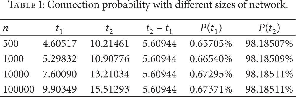
Figure 5 shows connection probability when . Table 1 demonstrates the values of , , , , and and corresponding values of and , for . For anyin the table, the obtained value . Of course, in a real network, the number of neighbors is integer, so 6 neighbors are needed. This example implies that, regardless of network size (number of nodes should be big enough), if the network connection probability is 0.66%, by increasing the communication range until each node obtains 6 more neighbors (namely, increasing communication range by 6 ), the network connection probability reaches at least 98.17%. Meanwhile, the network will be at least -connected.
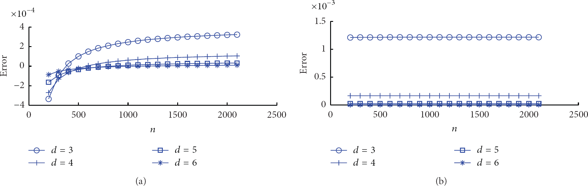
In order to validate Theorems 6 and 8, this paper calculates the error between theoretical results and approximation values with different n and b, as shown in Figure 6. The error of Theorem 6 is defined as , and the error of Theorem 8 is defined as . The errors for both theorems are very small, which indicate that both have a good approximation.
Connection probability with different sizes of network.
n
Network connection probability increases from to for .
Network connection probability when , and .
(a) The errors of Theorem 6; (b) the errors of Theorem 8.
4. Heterogenous Node Deployment in WSNs
In the last section, the obtained asymptotic results were based on the assumption that each node has the same communication range which is often not the case in practice. This section presents the connection probability when node communication range follows a normal distribution, that is, .
Formally, network model is reformulated as follows: n nodes are randomly and uniformly deployed in area A with density . Communication range of node i, denoted as , is i.i.d random variable and has normal distribution . Hence, the number of neighbors of the node, denoted as , is the Poisson random variable condition on parameter t, where . This model is analog to the so-called Cox process in which random variable is Poisson process where density itself is a stochastic process. Cox process is widely used in economics, for example, [14].
4.1. Connection Probability for Random Communication Range
denotes the expected value of a random variable V; therefore the expected neighbors of node are
In what follows, connection probability itself is researched. For , probability of node i having at least k neighbors is given by
For , is the probability that node i is not isolated. has log normal distribution. Therefore, the expected value and variance can be obtained via standard method:
For neighbors, the distribution of does not have a closed-form expression.
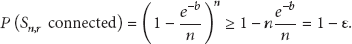
If n is big enough, the probability of network being k-connected is
Since parameter t is a random variable, is a random variable as well. Letting , because , so
Therefore the obstruction of connection probability of entire network is the node which has the minimal communication range.
is affected by several parameters: k, n, μ, and σ. Theorem 6 is used to decide μ. According to Theorem 6, the probability of the network being connected is at least 99.33% when . Let and take as average μ of communication range; for instance, if , then . In other words, 500 nodes with node communication range following normal distribution are deployed.
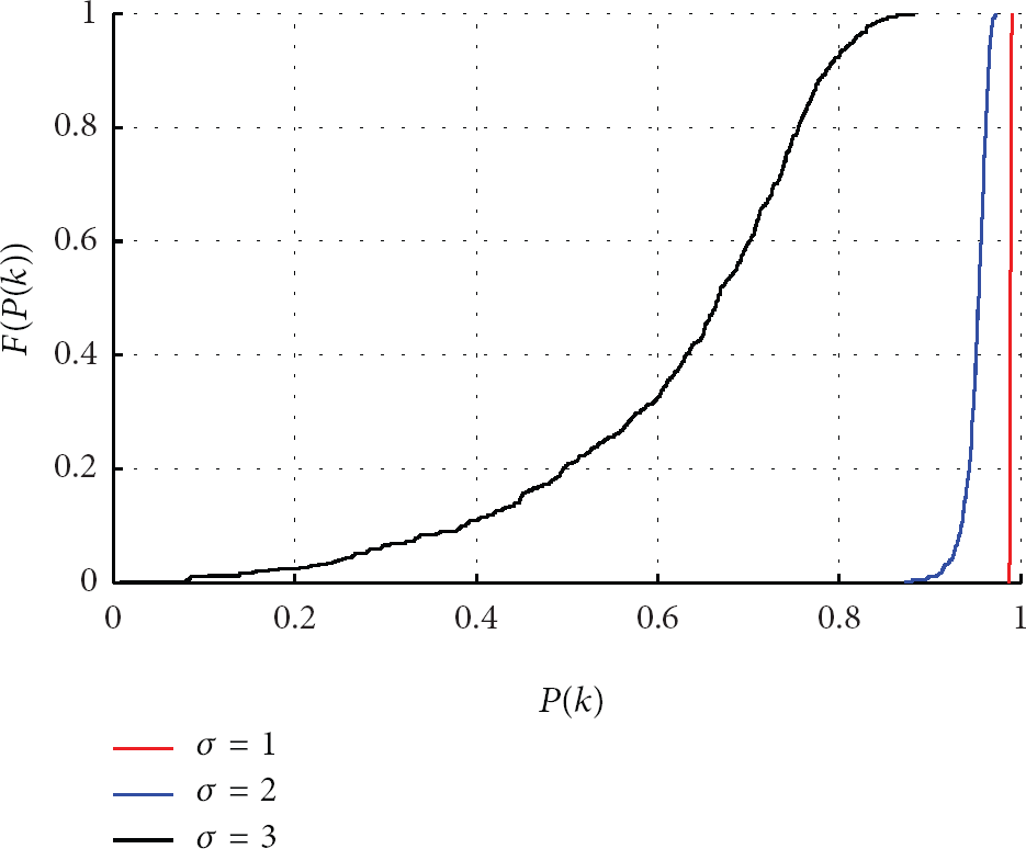
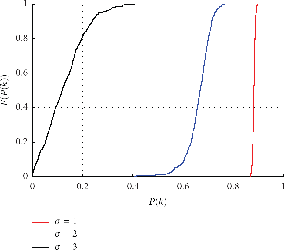
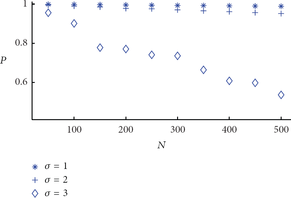
Our major concerns are the parameter σ which indicats communication range difference and k which shows the resilience capability. In order to study the changes of connection probability as parameters vary, the following simulations are performed: (1) cumulative distribution function (CDF) of is calculated after 500 runs with various σ and k, as shown in Figures 7 and 8; (2) given μ and σ, what is the probability of network being k-connected as the number of nodes deployed grows? This is done by computing average of after 500 runs for a given number of nodes, as illustrated in Figures 9 and 10; (3) how to choose the parameters in order to get the required connection probability. This is discussed in Section .
Cumulative distribution function (CDF) of when , and 3, , and .
Cumulative distribution function (CDF) of when , and 3, , and .
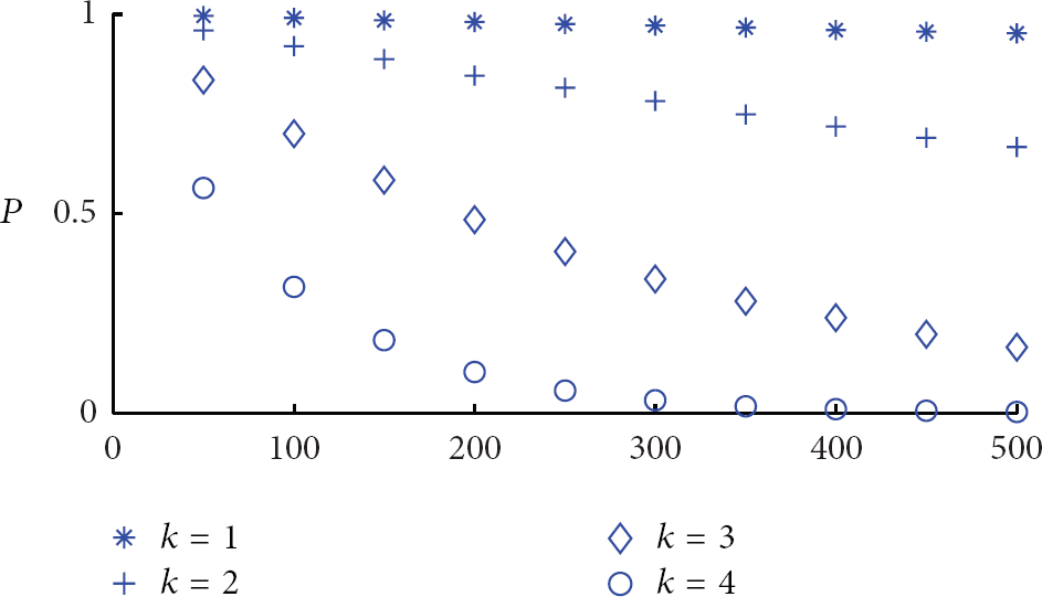
k-connected probability P when and , and 4.
Connection probability P when , and 3 and .
Figures 7 and 8 show the CDF of when σ and k change. The network probability is sensitive to standard deviation. As mentioned earlier, a single node that has small communication range can cause the whole network connection probability to be low. For instance, in Figure 8 when and , the probability of network being connected is almost sure less than 40%.
Figure 9 illustrates the connection probability as N nodes were deployed in network when and . Figure 10 shows the changes when and . Both figures show that the average of is the decreasing function of k, N, and σ. Network connection probability as network size growing is predictable. For instance, Figure 10 shows that the network average connection probability for is about 73% when the network has 250 nodes, but the probability falls to 55% if the network size is doubled. Figure 9 shows how the resilience performance decreases when network size grows or the probability decreases if higher resilience performance is required. For example, for networks which have 200 nodes, the probability that this network can tolerate 1, 2, and 3 (i.e., ) nodes failure are about 83%, 50%, and 10%, respectively.
4.2. Choose Distribution Parameter
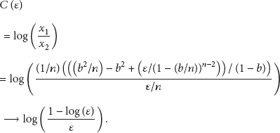
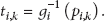
The simulations in Section 4.2 show with different parameters. In this section, it is addressed which distribution parameter(s) can maintain the given . This is helpful to choose appropriate parameters when network simulator is used to simulate real networks. According to (6), (22) is a monotonically increasing function of , and its inverse function is written as
Letting be an instance of , thus . The probability being greater than is given by
where is the probability density function of t. If the probability of a network required to keep network k-connected is at least , the corresponding probability for each node is at least
With formula (26)–(28), the required density function parameter of communication range for given can be calculated.
For example, 500 nodes are deployed in ; communication area is with mean . If the desired probability of the whole network being connected, that is, k-connected, is at least 90%. Standard deviation of this distribution is evaluated. For , according to (26) and (28), corresponding minimal range is . In order to make probability of greater than is high, for example, at least 95%, according to (27), . Therefore corresponding standard deviation σ should be no more than 0.93. This is useful in the case of using network simulator to choose appropriate parameters to design high probability connected networks. Figure 11 shows the required σ in order to make the network connection probability at least 90% when the number of nodes are different. Note that the node density is always 1.
Required σ for 90% connection probability when .
5. Related Works
Extensive studies have been done on the connection problem of networks. Many of them focus on how many neighbors or network density is needed so that a network connects with high probability, such as [15]; some construct network to satisfy connectivity [16, 17]; some works try to develop algorithms to preserve network connectivity or coverage, for example, [18–20], while some other works study other aspects of network connectivity, such as [21] which evaluates the quality of connectivity by measuring the reliability of link; it shows that the largest eigenvalue of the probabilistic connectivity matrix can serve as a good measure of the quality of network connectivity. When all the nodes of a region fail, [22] measures the number of connected components. This paper studies the connection probability when the network nodes are randomly deployed.
When nodes are randomly deployed, asymptotic upper and lower bounds of connection probability for both k-nearest neighbor and disk model have been studied [12]. For k-nearest neighbor, [23] concludes that, as , if each node is connected to less than neighbors, the network is disconnected with probability one, while, if neighbors are more than , the network is connected with probability one. Reference [24] finds that if , the network is not connected with high probability and if , then network is connected with high probability as . But for the directed network the upper and lower bounds are and , respectively. Reference [25] improves the upper bound to be . For disk model [26] states that 6 to 10 average numbers of neighbors almost make sure that network will be fully connected no matter how many nodes there are totally in the network. In [27], if communication range , then the network connection probability tends to be . Compared with [26], Table 1 in this paper shows that, when , at least neighbors are needed in order to make sure that network is connected with high probability. Besides, a result (Theorem 9) presented in our paper is the same as [27] but uses a totally different approach.
Reference [11] shows that, in k-nearest neighbor model by increasing, network becomes s-connected very shortly after it becomes connected, where . Reference [28] proves one conjecture in [24] that, in k-nearest neighbor model for every and n sufficiently large, there exists such that, if the network has k-connected probability ɛ, then -connected probability is bigger than . This paper improves the results in [11], obtaining an explicit expression for disk model, that is, , where . The corollary in this paper proves that the result for disc model has a similar form presented in [28].
Nodes having the same communication range usually are not true in reality. In order to make the model more accurate, [8, 29] utilize irregular radio to model real nodes. The connectivity for heterogenous networks has been well studied; for example, [16, 30] investigate the relay node placement problem such that network is the k-connected. The authors in [31] assumes that node communication radius of node i is i.i.d. random variable with normal probability density . Reference [32] adopts the model that Poisson intensity is given by a normal distribution; then it obtains the asymptotic bound of range that all nodes in this area are connected to the origin. Reference [33] considers nodes are placed according to a shot-noise Cox process rather than uniform deployment. This paper employs the stochastic methods to characterize heterogenous network. In this paper the density is maintained constant, but the node communication range is normal distribution.
6. Conclusion and Future Works
When deploying many WSNs nodes, one of the key problems is whether all nodes in the network are connected to other nodes. Isolated nodes will be useless for applications. This paper presents the results on how the network connection probability changes as the communication range varies in randomly and uniformly distributed homogenous and heterogenous WSNs. In case of network with all nodes having the same communication range, through theory derivation and validation, this paper proves that, regardless of network size, the network connection probability increases from to by increasing constant communication range of each node. As the example shows in Section 3.2, regardless of network size, if the network connection probability is 0.66%, by increasing the communication range until each node obtains 6 more neighbors, the network connection probability reaches at least 98.17%. On the other hand, this paper shows that, once network is connected, it also becomes -connected with high probability, which makes the network resilient against node failures because there are alternative paths between any two distinct nodes.
In case each node communication range is i.i.d random variable which has normal distribution, this paper analyzes the connection probability by simulation. This paper shows that network connection probability is determined by the distribution parameters and the network size, especially sensitive to standard deviation. The reason is that the network connection probability is dependent on the node that has minimal communication range. It implies that it needs to take care of the node which has minimal communication range because it is the bottleneck of the whole network. The network will become disconnected if they fail. With the same configuration, the resilience capability decreases when network size grows. Besides, given the required connection probability, this paper develops one method to decide the distribution parameter of communication range. This method can be used to choose appropriate distribution parameter of communication range for network simulators or real deployments.
In some circumstances, a full connected network is impractical and not necessary. One would be more interested in the giant connected component which contains most nodes of entire network are connected. More specifically, the relation between the giant connected component and the communication range distribution is what is wanted to be learnt. It is a percolation problem with random communication range. Percolation occurs when a node belongs to infinite component with none-zero possibility. The critical intensity is defined as the minimum intensity in which percolation occurs. For disk model, the bound for critical intensity is known (e.g., [34]) but for variable radius is unknown. Therefore, studying the percolation problem with i.i.d communication range (or radius) will be our future work. On the other hand, the degree of the node obeys Poisson distribution in this paper. It has been found that many networks, such as the World Wide Web, the Internet, airplanes connection networks, some biological systems, and international ownership network, have power-law degree distribution with an exponent that ranges between and [35]. Our future work will center on connection probability with a more accurate model.
References
1.
AzizA. A.SekerciogluY. A.FitzpatrickP.IvanovichM.A survey on distributed topology control techniques for extending the lifetime of battery powered wireless sensor networksIEEE Communications Surveys and Tutorials20131511211442-s2.0-8485922430910.1109/SURV.2012.031612.00124
2.
ZhuC.ZhengC.ShuL.HanG.A survey on coverage and connectivity issues in wireless sensor networksJournal of Network and Computer Applications20123526196322-s2.0-8485622552110.1016/j.jnca.2011.11.016
3.
AtzoriL.IeraA.MorabitoG.The internet of things: a surveyComputer Networks20105415278728052-s2.0-7795687712410.1016/j.comnet.2010.05.010
4.
SahaI.SambasivanL. K.GhoshS. K.PatroR. K.Distributed fault-tolerant topology control in wireless multi-hop networksWireless Networks2010166151115242-s2.0-7795786248210.1007/s11276-008-0133-2
5.
PintoP. C.WinM. Z.Communication in a poisson field of interferers—part I: interference distribution and error probabilityIEEE Transactions on Wireless Communications201097217621862-s2.0-7795474792110.1109/TWC.2010.07.060438
6.
AdrianBondyMurtyU. S. R.Graph Theory2008Berlin, GermanySpringer
7.
ChongP. K.KimD.Surface-level path loss modeling for sensor networks in flat and irregular terrainACM Transactions on Sensor Networks201392132
8.
ZhuK.Ad hoc network deployment accommodating short and uncertain transmission rangeProceedings of the 9th ACM International Symposium on Mobility Management and Wireless Access (MobiWac ′11)November 2011New York, NY, USA1011082-s2.0-8305517714110.1145/2069131.2069149
9.
BettstetterC.On the minimum node degree and connectivity of a wireless multihop networkProceedings of the 3rd ACM International Symposium On Mobile Ad Hoc Networking & Computing (MOBIHOC ′02)June 2002Lausanne, Switzerland80912-s2.0-0242696202
10.
PenroseM. D.On k-connectivity for a geometric random graphRandom Structures and Algorithms19991521451642-s2.0-0033471867
11.
BalisterP.BollobásB.SarkarA.WaltersM.Highly connected random geometric graphsDiscrete Applied Mathematics200915723093202-s2.0-5634909931210.1016/j.dam.2008.03.001
12.
BalisterP.SarkarA.BollobsB.Percolation, connectivity, coverage and colouring of random geometric graphsHandbook of Large-Scale Random Networks2008Berlin, GermanySpringer117142
DelattreS.RobertC. Y.RosenbaumM.Estimating the efficient price from the order flow: a Brownian Cox process approachStochastic Processes and Their Applications2013123726032619
15.
CaiH.JiaX.ShaM.Critical sensor density for partial connectivity in large area wireless sensor networksACM Transactions on Sensor Networks201174, article 352-s2.0-7995250751810.1145/1921621.1921629
16.
HanX.CaoX.LloydE. L.ShenC.-C.Fault-tolerant relay node placement in heterogeneous wireless sensor networksIEEE Transactions on Mobile Computing2010956436562-s2.0-7794987545610.1109/TMC.2009.161
17.
BredinJ. L.DemaineE. D.HajiaghayiM.RusD.Deploying sensor networks with guaranteed capacity and fault toleranceProceedings of the 6th ACM International Symposium on Mobile Ad Hoc Networking and Computing (MOBIHOC ′05)May 2005Urbana-Champaign, III, USA3093192-s2.0-2984445616310.1145/1062689.1062729
18.
YuJ.RenS.WanS.YuD.WangG.A stochastic coverage scheduling algorithm in wireless sensor networksInternational Journal of Distributed Sensor Networks201220121174650110.1155/2012/746501
19.
MiZ.YangY.DingH.Self-organized connectivity control and optimization subjected to dispersion of mobile ad hoc sensor networksInternational Journal of Distributed Sensor Networks201220121567243610.1155/2012/672436
20.
BishopM.CarvalhoM.FordR.MayronL. M.Resilience is more than availabilityProceedings of the New Security Paradigms Workshop (NSPW ′11)September 2011Marin County, Calif, USA951042-s2.0-8485568189010.1145/2073276.2073286
21.
DasguptaS.MaoG.On the quality of wireless network connectivity500Proceedings of the IEEE Global Communications Conference (GLOBECOM ′12)December 201250537
22.
BanerjeeS.ShirazipourazadS.GhoshP.SenA.Beyond connectivity—new metrics to evaluate robustness of networksProceedings of the IEEE 12th International Conference on High Performance Switching and Routing (HPSR ′11)July 20111711772-s2.0-8005273139310.1109/HPSR.2011.5986022
23.
XueF.KumarP. R.The number of neighbors needed for connectivity ofwireless networksWireless Networks20041021691812-s2.0-104228903110.1023/B:WINE.0000013081.09837.c0
24.
BalisterP.BollobásB.SarkarA.WaltersM.Connectivity of random k-nearest-neighbour graphsAdvances in Applied Probability20053711242-s2.0-1774439265510.1239/aap/1113402397
25.
WaltersM.Small components in k-nearest neighbour graphsDiscrete Applied Mathematics20121601314203720472-s2.0-8486056160610.1016/j.dam.2012.03.033
26.
NiJ.ChandlerS. A. G.Connectivity properties of a random radio networkIEE Proceedings199414142892962-s2.0-002847988110.1049/ip-com:19941197
27.
PenroseM. D.Random Geometric Graphs2003Oxford, UKOxford University Press
28.
Falgas-RavryV.WaltersM.Sharpness in the k-nearest neighbors ranmdom geometric graph modelAdvances in Applied Probability2012443617634
29.
ChenjiH.StoleruR.Mobile sensor network localization in harsh environmentsProceedings of the 6th IEEE International Conference on Distributed Computing in Sensor Systems2010Santa Barbara, Calif, USASpringer244257
30.
DandekarD. R.DeshmukhP. R.Relay node placement for multi-path connectivity in heterogeneous wireless sensor networksProcedia Technology20124732736
31.
GuanZ.-H.DingL.KongZ.-M.Multi-radius geographical spatial networks: statistical characteristics and application to wireless sensor networksPhysica A201038911982042-s2.0-7034946772510.1016/j.physa.2009.09.021
32.
BalisterP.BollobasB.SarkarA.WaltersM.Connectivity of a Gaussian networkInternational Journal of Ad Hoc and Ubiquitous Computing2008332042132-s2.0-4434918028010.1504/IJAHUC.2008.018407
33.
AlfanoG.GarettoM.LeonardiE.MartinaV.Capacity scaling of wireless networks with inhomogeneous node density: lower boundsIEEE/ACM Transactions on Networking2010185162416362-s2.0-7795815443610.1109/TNET.2010.2048719
34.
NgS. C.MaoG.AndersonB. D. O.Analytical bounds on the critical density for percolation in wireless multi-hop networksProceedings of the 54th Annual IEEE Global Telecommunications Conference Energizing Global Communications (GLOBECOM ′11)December 2011Houston, Tex, USA162-s2.0-8485721713110.1109/GLOCOM.2011.6133604
35.
VitaliS.GlattfelderJ. B.BattistonS.The network of Global corporate controlPLoS One20116102-s2.0-7995963873810.1371/journal.pone.0025995e25995