Towards Robust Routing in Three-Dimensional Underwater Wireless Sensor Networks

Abstract

The areas of three-dimensional (3D) underwater wireless sensor networks (UWSNs) have attracted significant attention recently due to their applications in detecting and observing phenomena that cannot be adequately observed by means of two-dimensional UWSNs. However, designing routing protocols for UWSNs is a challenging task because path breakage occurs frequently due to uncertain node and link failures. In this paper, we present a Robust Routing Protocol (RRP) that aims to achieve robustness under harsh underwater conditions of 3D UWSNs. In RRP, each sensor has a data structure called backup bin, which allows to construct main backup links and auxiliary backup links for repairing failed links and ensuring normal data delivery. Moreover, sensor nodes can also enlarge their transmission range to build new links when the main routing path is not reachable through backup links. Simulation results show that the proposed protocol can reduce node and link failures' impact on metrics of packet delivery ratio, network throughput, energy consumption, and average end-to-end delay.

1. Introduction

Underwater wireless sensor networks (UWSNs) have a lot of potential application areas such as oceanographic data collection, disaster prevention, pollution monitoring, offshore exploration, and military surveillance [1–3]. Radio frequency (RF) signals suffer from severe attenuation in water and have been successfully deployed only at very low frequencies, involving large antenna and high transmission power. Hence, acoustic signals have been used for wireless communication in current underwater physical layer, which has challenges to be overcome such as long propagation delay resulting from low speed of sound propagation, severely limited bandwidth, and time-varying multipath propagation [4, 5]. All the above distinct features of UWSNs give birth to new challenges areas for every level of the network protocol suite. UWSNs consist of a variable number of sensors and vehicles that are deployed to perform collaborative monitoring tasks over a given area. To achieve this objective, sensors and vehicles self-organize in an autonomous network that can adapt to the characteristics of the underwater environment.

Three-dimensional (3D) UWSNs are used to detect and observe phenomena that cannot be adequately observed by means of ocean bottom underwater sensor nodes, that is, to perform cooperative sampling of the 3D ocean environment [6–8]. In 3D UWSNs, sensors float at different depths to observe a given phenomenon. Many problems arise with 3D UWSNs that need to be solved in order to enable underwater monitoring in the new environment. Among them, providing efficient routing is a very challenging task due to the unique characteristics of 3D UWSNs. 3D UWSNs must rely on underwater acoustic communications because high-frequency radio signals used in traditional ground-based sensor networks can be rapidly absorbed by water. Therefore, many research results in land-based sensor networks as well as traditional ad hoc networks cannot be applied to 3D UWSNs directly, which requires new routing protocol to be designed for the new features of the 3D UWSNs in order to ensure that the performance can meet the actual underwater environmental needs.

According to their architectures, the routing protocols of 3D UWSNs can be divided into three categories: location-based routing, flat routing, and hierarchical routing [9, 10]. Location-based routing has good scalability, but it requires a positioning system or positioning algorithm to help the nodes to calculate the location information. Flat routing protocols have better robustness, but the excessive overhead for maintaining routing information restricts their application to small-scale underwater acoustic circumstances. Hierarchical routing also has good scalability, but the cluster maintenance overhead and the failure of key nodes will affect the routing efficiency.

In 3D UWSNs, communication links face high bit error rate, temporary losses, or even permanent failure. Moreover, the impact of node failure is more severe than that of link failure because even a single node failure is logically equivalent to several concurrent link failures. In this paper, we propose a Robust Routing Protocol (RRP) that addresses some of the major requirements imposed by 3D UWSNs including high robustness combined with energy-efficient communication. Since 3D UWSNs are made up of expensive sensor nodes and they operate in harsh underwater environments, the likely possibility of node or link failures must be considered. In RRP, each sensor has a data structure called backup bin, which has been utilized to construct main backup links and auxiliary backup links together with routing table for repairing routing path and ensuring normal data delivery. As geographic routing protocol, RRP does not require state information on the sensor nodes and only a small fraction of the nodes are involved in routing to ensure robust operation for surveillance and monitoring applications.

The remainder of the paper is organized as follows. Section 2 presents a brief overview of related work, while Section 3 introduces the technical details of our routing protocol. Performance evaluation is described in Section 4. Finally, we conclude the paper in Section 5.

2. Related Work

The underwater environment introduces difficulties in designing efficient routing protocols not experienced terrestrially, such as transmission loss due to geometric spreading and absorption by the ocean [11, 12]. Tan et al. [13] proposed a new protocol based on hop-by-hop hybrid implicit/explicit acknowledgment scheme which is proposed for a multihop UWSN. In this protocol, data packets forwarded by downstream nodes can work as implicit ACKs for previous transmitted data packets. Vahdat and Becker [14] proposed Epidemic Routing (ER) protocol where each node replicates a packet to every encountered node. ER can utilize every opportunity to deliver a packet to the destination and maximize successful delivery ratio and minimize average end-to-end delay in unconstrained networks. However, this routing protocol consumes too many resources that make it not desirable in resource-constrained networks such as UWSNs. Pompili et al. [15] introduced two distributed routing algorithms for delay-insensitive and delay-sensitive applications, respectively, with the objective of minimizing the energy consumption taking the varying condition of the underwater channel and the different application requirements into account.

Vector-based forwarding (VBF) [16] is a geographic approach, which allows the nodes to weigh the benefit to forward packets and reduce energy consumption by discarding low benefit packets. Therefore, over a multihop path, only the nodes that are located within a pipe of given width between the source and the destination are considered for relaying. However, in the areas of low density of nodes, VBF may not find the path close to the routing vector. Similarly, Jornet et al. proposed Focused-Beam Routing (FBR) [17] protocol that is suitable for networks containing both static and mobile nodes. The objective of FBR is to determine which nodes are candidates for relaying. Candidate nodes are those that lie within a cone of angle $\pm \theta /2$ emanating from the transmitter towards the final destination. An RTS/CTS handshake is set up to isolate closer nodes within this cone. If a node determines that it is within the transmitter's cone, it will respond to the RTS. Those nodes that are outside the cone will not respond. A theoretical argument supporting geographic routing has been discussed in [18] based on simple propagation and energy consumption models for underwater networks. The study shows that an optimal number of hops along a path exist and that increasing the number of hops by choosing closer relays is preferable with respect to keeping the route shorter. In view of this, several position-based routing algorithms are proposed and compared; results show that selecting relays closer than a given maximum distance before seeking farther ones achieves in fact optimal energy consumption.

Depth-Based Routing (DBR) [19] can handle network dynamics efficiently without the assistance of a localization service. DBR forwards data packets greedily towards the water surface (i.e., the plane of data sinks). In DBR, a data packet has a field that records the depth information of its recent forwarder and is updated at every hop. But DBR has only greedy forwarding mode, which alone is not able to achieve high delivery ratios in sparse areas. A similar idea can be found in [20], a hydraulic pressure-based anycast routing protocol that exploits the measured pressure levels to route data to surface buoys where relays are chosen based on a weighted average of advancement towards the sources and probability of packet delivery, and an efficient underwater dead end recovery method is added to handle the absence of a relay node at lower depth than the current packet holder. In order to remove the constraints imposed by special hardware (like every node should be equipped with depth or pressure sensor, which not only increase the cost of the network but also become a burden for extra energy consumption), Ayaz and Abdullah [21] proposed a Hop-by-Hop Dynamic Addressing-Based (H2-DAB) routing protocol to provide scalable and time-efficient routing for UWSN. The H2-DAB routing protocol does not require any dimensional location information or any extra specialized hardware compared with many other routing protocols in the same area. However, the problem of multihop routing still exists as it is based on multihop architecture, where nodes near the sinks drain more energy because they are used more frequently. Noh et al. [22] proposed a Void-Aware Pressure Routing (VAPR) protocol that uses sequence number, hop count, and depth information embedded in periodic beacons to set up next-hop direction and to build a directional trail to the closest sink. VAPR employs periodical beacon messages to identify the direction of each node in a heuristic manner. The direction is set as up when a beacon is received from a shallower depth node; otherwise, it is set as down. When multiple direction cues are received from different sinks, the direction cue with the minimal hop count is chosen. Also, a node's next-hop data forwarding direction is set based on the beacon sender's data forwarding direction. VAPR employs a multisink structure to prevent a rapid battery drain in the nodes closer to the sinks. Moreover, it can handle the void problem with a heuristic method. However, each node in VAPR requires the knowledge of 2-hop connectivity and neighboring nodes' pairwise distances. In addition, the enhanced beaconing component should be repeated in a short interval (usually 50 seconds at a time), which causes a significant increase in the network overhead.

Packet redundancy and multiple paths can be exploited in order to increase the reliability of UWSNs. Ayaz et al. [23] provided a two-hop acknowledgment reliability model in order to insure the reliable data deliveries to the surface sinks, where two copies of the same data packet are maintained in the network without extra burden on the available resources. A relay node that has data packets to forward will not reply the acknowledgment until it cannot find the next hop towards the destination. But if a node is unable to find the next hop due to any failure, or even if it is lost, then packets in the buffer are not considered lost. All the nodes that send the data packets towards this node will wait for a certain amount of time before trying again for the next hop. Xu et al. [24] proposed a Multiple-Path Forward Error Correction (M-FEC) approach that integrated multiple-path communications and Hamming Coding to eliminate retransmission and enhance reliability in underwater sensor networks. Moreover, a Markov model and a dynamical decision and feedback scheme were developed to decrease the number of the paths in order to save energy and ensure the desirable packet error rate. However, M-FEC may cause much long delay because of additional process of encoding and decoding the data packets, and it does not tackle the issues of node and link failures.

3. Proposed Scheme

3.1. Network Model and Definitions

We consider that 3D UWSNs are composed of a certain number of sensor nodes uniformly scattered in monitoring fields. We present a generic model for a 3D UWSN that is represented by $G=(V,E)$ with n sensor nodes. Every sensor node has the same transmission range and is assigned with a triplet of coordinates $(x,y,z)$ , where each coordinate represents the hop distance of the node from one anchor. We also assume that all sensor nodes know their own locations through a certain localization service [25]. Such assumption is justified in underwater systems where fixed bottom-mounted nodes have location information upon deployment. In fact, the underwater localization is a nontrivial task for which relatively very few options are available. For example, employing global positioning system (GPS) does not work well because radio frequency (RF) waves are heavily attenuated in underwater environment. Many researchers have proposed a variety of localization schemes and techniques to address this issue specially [26, 27]. It is not always feasible to deploy anchor nodes at the sea floor for deep water environment. In this case, mobile beacon nodes such as autonomous underwater vehicles (AUVs), which are equipped with internal navigation systems, are exploited as reference nodes to assist in corresponding distributed localization algorithms. This paper takes advantage of these research results as existing preconditions. Moreover, we also consider symmetric links; that is, for any two nodes $s_u$ and $s_v$ , $s_u$ reaches $s_v$ if and only if $s_v$ reaches $s_u$ . Each node can either transmit or receive data packet.

Definition 1.

The function $\delta (u,v)$ defines the distance between two nodes $s_u$ and $s_v$ in a 3D Euclidean space as

$$\begin{array}{cc}& \delta :N\times N⟶\mathrm{\Gamma }:\delta (u,v),\\ \delta \left(u,v\right)=\sqrt{{\left(u_x-v_x\right)}^{\mathrm{2}}+{\left(u_y-v_y\right)}^{\mathrm{2}}+{\left(u_z-v_z\right)}^{\mathrm{2}}}.\end{array}$$

(1)

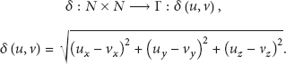
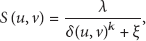
All sensor nodes have two transmission ranges $r_{\mathrm{norm}}$ (normal transmission range) and $r_{\max }$ (maximal transmission range). The normal transmission range is used for regular routing process with less energy usage, while the maximal transmission range is used to counteract the negative influence of node and link failures with more energy consumption when necessary. Two nodes $s_u$ and $s_v$ are neighbors and connected by a link if $\delta (u,v)<r_{\mathrm{norm}}$ . When the distance of two sensor nodes is equal or shorter than $r_{\mathrm{norm}}$ , the receiving rate is 1. When the distance is larger than $r_{\mathrm{norm}}$ but still within the range of $r_{\max }$ , then the receiving rate is between 0 and 1. Generally, the receiving rate of nodes $s_u$ and $s_v$ is calculated as

$$\begin{array}{cc}& \eta (u,v)=\{\begin{array}{cc}\mathrm{1},\hfill & \delta \left(u,v\right)\le r_{\mathrm{norm}},\hfill \\ \frac{r_{\max }-\delta (u,v)}{r_{\max }-r_{\mathrm{norm}}},\hfill & r_{\mathrm{norm}}<\delta \left(u,v\right)<r_{\max },\hfill \\ \mathrm{0},\hfill & \delta \left(u,v\right)\ge r_{\max }.\hfill \end{array}\end{array}$$

(2)

Note that even at a short distance from the transmitter to the receiver, the receiving rate is still lower than 1. The reason is that underwater acoustic channels are affected by many factors such as path loss, noise, multipath fading, and Doppler spread. All these factors cause a high bit error rate in underwater environment. For simplicity, the receiving rate in the normal transmission range is assumed to be 1, which will not affect the performance comparison of different routing protocols. In other cases, the receiving rate is calculated according to formula (2).

Consider two sensor nodes at minimum hop distance h; there exist two values $u(h)$ and $v(h)$ such that the Euclidean distance $\delta (u,v)$ between the two nodes is bounded; that is, $u(h)\le \delta (u,v)\le v(h)$ . The quality of the bounds depends on the network density ρ. In particular for each $h>0$ holds

$$\begin{array}{cc}& \underset{\rho \to \infty }{\lim }v\left(h\right)-u\left(h\right)=r_{\mathrm{norm}},\end{array}$$

(3)

where $r_{\mathrm{norm}}$ is the normal transmission range of the sensor nodes.

Sensing devices generally have widely different theoretical and physical characteristics. Thus, numerous models of varying complexity can be constructed based on application needs and device features. However, for most kinds of sensors, the sensing ability diminishes as distance increases.

Definition 2.

Given a source sensor node $s_u$ and a destination sensor node $s_v$ , then the sensor model is defined as

$$\begin{array}{cc}& S\left(u,v\right)=\frac{\lambda }{\delta {\left(u,v\right)}^k+\xi },\end{array}$$

(4)

with $\lambda >0$ and $\xi >0$ , where λ is the signal amplitude, k is the sensor technology-dependent parameter, and ξ is a predefined parameter for handling the situation when the source node and the destination node locate at the same position.

Underwater wireless sensor nodes have been equipped with sensing devices. They collect data from the external environment and transmit these data by one or multihop to the sink node. Sink node is the node that generates data aggregation results and also the target location of the data transmission. A routing path p that consists of m sensor nodes can be expressed as $p=\{s_1,s_2,\dots ,s_m\}$ , where $(s_i,s_{i+\mathrm{1}})\in E$ , $i\in [1,\dots ,m-1]$ , and the length of path p is $L(p)$ . If there exist n paths from the source node to the sink node, then these paths can be expressed as $\chi =\{p_1,p_2,\dots ,p_n\}$ with length $L(\chi )=\sum L(p_i)$ .

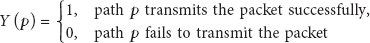
In order to build nodes' state model, we use a random variable $X(u)$ to denote the node $s_u$ 's state and $X(u)$ obeys the following Bernoulli distribution:

$$\begin{array}{cc}& X\left(u\right)=\{\begin{array}{cc}\mathrm{1},\hfill & s_u\mathrm{\hspace{0.17em}\hspace{0.17em}}\text{transmits}\mathrm{\hspace{0.17em}\hspace{0.17em}}\text{the}\mathrm{\hspace{0.17em}\hspace{0.17em}}\text{packet}\mathrm{\hspace{0.17em}\hspace{0.17em}}\text{successfully},\hfill \\ \mathrm{0},\hfill & s_u\mathrm{\hspace{0.17em}\hspace{0.17em}}\text{fails}\mathrm{\hspace{0.17em}\hspace{0.17em}}\text{to}\mathrm{\hspace{0.17em}\hspace{0.17em}}\text{transmit}\mathrm{\hspace{0.17em}\hspace{0.17em}}\text{the}\mathrm{\hspace{0.17em}\hspace{0.17em}}\text{packet}.\hfill \end{array}\end{array}$$

(5)

Definition 3.

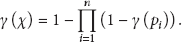
The probability $\text{Pr}(X(u)=1)$ for a sensor node $s_u$ to transmit a packet successfully is called $s_u$ 's packet transmit rate and is denoted by $\gamma (s_u)$ .

The state model for a routing path $p=\{s_1,s_2,\dots ,s_m\}$ is represented by $Y(p)$ and $Y(p)$ obeys the following distribution:

$$\begin{array}{cc}& Y\left(p\right)=\{\begin{array}{cc}\mathrm{1},\hfill & \text{path}\mathrm{\hspace{0.17em}\hspace{0.17em}}p\hspace{0.17em}\hspace{0.17em}\text{transmits}\mathrm{\hspace{0.17em}\hspace{0.17em}}\text{the}\mathrm{\hspace{0.17em}\hspace{0.17em}}\text{packet}\mathrm{\hspace{0.17em}\hspace{0.17em}}\text{successfully},\hfill \\ \mathrm{0},\hfill & \text{path}\mathrm{\hspace{0.17em}\hspace{0.17em}}p\hspace{0.17em}\hspace{0.17em}\text{fails}\mathrm{\hspace{0.17em}\hspace{0.17em}}\text{to}\mathrm{\hspace{0.17em}\hspace{0.17em}}\text{transmit}\mathrm{\hspace{0.17em}\hspace{0.17em}}\text{the}\mathrm{\hspace{0.17em}\hspace{0.17em}}\text{packet}\hfill \end{array}\end{array}$$

(6)

and $Y(p)={\prod }_{i=\mathrm{1}}^{m}X(i)$ . If the failure probabilities for the nodes in path p are independent, $Y(p)$ also obeys the Bernoulli distribution and the packet transmit rate of path p is denoted by $\gamma (p)$ , which is equal to ${\prod }_{i=\mathrm{1}}^m\gamma (s_i)$ . If there exist n paths $\chi =\{p_1,p_2,\dots ,p_n\}$ from the source node to the sink node, the packet transmit rate of path χ is calculated as

$$\begin{array}{cc}& \gamma \left(\chi \right)=\mathrm{1}-{\displaystyle \prod }_{i=\mathrm{1}}^n\left(\mathrm{1}-\gamma \left(p_i\right)\right).\end{array}$$

(7)

Acoustic signal has different transmission modes in shallow water (where the depth of the water is less than 100 meters) and deep water (where the depth of the water is more than 100 meters). In shallow water, the transmission of the acoustic signal is limited to a cylindrical area from bottom to the surface. The energy consumption for transmission in the shallow water is calculated as

$$\begin{array}{cc}& {\epsilon }_t=\mathrm{10}\hspace{0.17em}{\log }_{\mathrm{2}}\delta \left(u,v\right)+\alpha \delta \left(u,v\right)·\mathrm{1}{\mathrm{0}}^{\mathrm{3}},\end{array}$$

(8)

where $\delta (u,v)$ denotes the Euler distance between the sender and the receiver and α is the absorption coefficient.

In deep water, the transmission of the acoustic signal is mainly with spherical diffusion. The energy consumption is caused by spherical diffusion and water absorption, which can be calculated as

$$\begin{array}{cc}& {\epsilon }_t=\mathrm{20}\hspace{0.17em}{\log }_{\mathrm{2}}\delta \left(u,v\right)+\alpha \delta \left(u,v\right)·\mathrm{1}{\mathrm{0}}^{\mathrm{3}}.\end{array}$$

(9)

3.2. Packets Reception Strategies

We denote the size of the transmit node's buffer pool by buf and $z_{ij}$ is the stochastic variable that represents the number of packets transmitted from the source node $s_i$ to the destination node $s_j$ per slot; then we get $z_{i·}={\sum }_{j=\mathrm{1}}^n{z}_{ij}$ . The number of packets from all sources to the destination node $s_j$ per slot is $z_{·j}={\sum }_{i=\mathrm{1}}^n{z}_{ij}$ . We denote by $x_{ij}$ the number of packets that $s_i$ retransmits to the destination node $s_j$ ; then the total number of retransmissions for $s_i$ is $x_{i·}={\sum }_{j=\mathrm{1}}^n{x}_{ij}$ and the total number of retransmitted packets to the destination node $s_j$ is $x_{·j}={\sum }_{i=\mathrm{1}}^n{x}_{ij}$ . In the symmetric model, we get

$$\begin{array}{cc}& E\left[z_{i·}\right]=E\left[z_{·j}\right]=z,\hspace{1em}\forall i,j=\mathrm{0,1},\dots ,n,\\ E\left[x_{i·}\right]=E\left[x_{·j}\right]=x,\hspace{1em}\forall i,j=\mathrm{0,1},\dots ,n.\end{array}$$

(10)

The First In First Out (FIFO) reception strategy selects the packet in the rightmost position of the current slot for reception. If there are several packets in the rightmost nonempty position, one is chosen deterministically. Intuitively, this strategy can be expected to have the least packet loss, as it selects the packet that has the shortest time still to spend in the receiver. Suppose the receiver is in state $S_t$ , $t=\mathrm{0,1},\dots ,d$ , we build a discrete time Markov chain with $d+1$ states $S_0,S_1,S_2,\dots ,S_d$ . The chain changes state every $d+1$ received slots according to the arriving distribution $z_{·j}$ . Then the matrix of transition probabilities $p_{ik}$ is calculated as

$$\begin{array}{cc}& p_{ik}={{\displaystyle \sum }}_{z_{·j}\mid S_i\to S_k}P\left(z_{·j}\right),\hspace{1em}\forall i,k=\mathrm{0,1},\mathrm{2},\dots ,d.\end{array}$$

(11)

Let $\{{\pi }_i\mid i=\mathrm{0,1},\dots ,d\}$ be the steady state of the model; then the packet retransmission distribution $P(x_{·j}=k)$ is calculated as

$$\begin{array}{cc}& P(x_{·j}=k)={{\displaystyle \sum }}_{i=\mathrm{0}}^d{\pi }_i·x_{ik},\hspace{1em}\forall k=\mathrm{0,1},\dots ,n.\end{array}$$

(12)

Suppose the probability of packet rejection is α, then the reception position distribution for a received packet ${\rho }_k$ is calculated as

$$\begin{array}{cc}& {\rho }_k=\frac{\mathrm{1}}{\mathrm{1}-\alpha }{{\displaystyle \sum }}_{i=\mathrm{0}}^d{\pi }_i·p_{ik},\hspace{1em}\forall k=\mathrm{0,1},\dots ,n.\end{array}$$

(13)

The Last In First Out (LIFO) packets reception strategy selects the packet in the leftmost position of the current slot for reception. If several packets are in the leftmost nonempty position, one is chosen deterministically. Intuitively, this strategy is the easiest to implement, although it may exhibit the worst behavior in terms of packet loss since it selects the packet that has the longest time still to spend in the receiver. In LIFO, the packet retransmission distribution $P(x_{·j}=k)$ is calculated as

$$\begin{array}{cc}& P(x_{·j}=k)={{\displaystyle \sum }}_{z_{·j}\mid S_i\to S_k}^{d}P\left(z_{·j}\right),\hspace{1em}\forall k=\mathrm{0,1},\dots ,n.\end{array}$$

(14)

Suppose the probability of packet rejection is β, then the reception position distribution for a received packet ${\rho }_k$ is calculated as

$$\begin{array}{cc}& {\rho }_k=\frac{\mathrm{1}}{\mathrm{1}-\beta }{{\displaystyle \sum }}_{z_{·j}}P\left(z_{·j}\right),\hspace{1em}\forall k=\mathrm{0,1},\dots ,n.\end{array}$$

(15)

3.3. Routing Protocol

RRP consists of two phases: route discovery process and route maintenance process. During the process of route discovery, each packet carries the positions of the source node, the target node, and the relay node (i.e., the node that transmits this packet). Upon receiving a packet, a node computes the gravities of its neighbor nodes and chooses the neighbor with maximal gravity value to be the relay node that is in charge of forwarding the data packet.

Definition 4.

Given a sensor node $s_i$ and its neighbor node $s_j$ , the gravity function from $s_i$ to $s_j$ is defined as $G(\overrightarrow{ij})$ and its value is calculated as

$$\begin{array}{cc}& \left|G\left(\overrightarrow{ij}\right)\right|=\frac{{\epsilon }_i·{\epsilon }_j·\cos (A/\upsilon )}{\delta {\left(i,j\right)}^{\mathrm{2}}}\end{array}$$

(16)

with ${\epsilon }_i$ , ${\epsilon }_i>0$ and $\upsilon >2$ , where ${\epsilon }_i$ and ${\epsilon }_j$ denote the residual energy of sensor nodes $s_i$ and $s_j$ , A is the intersection angle between the direction of $s_i$ to $s_j$ and the direction of $s_i$ to $s_t$ (the target node), and a predefined parameter υ is used to adjust the impact of neighbor's direction angle on the gravity value.

The process of selecting a neighbor node as the relay node to forward a packet to a sink node is illustrated in Figure 1.

Figure 1

Relay node selection.

After sensor node $s_i$ receives a packet, it calculates gravity values of all neighbors within the normal transmission range $r_{\mathrm{norm}}$ to the sink node $s_t$ and the neighbor node with the maximum gravity value is selected as the relay node to forward the packet. The transmission space of $s_i$ is a sphere centered at this node as we address 3D UWSN in this paper. In order to save energy, every sensor node only adopts $r_{\mathrm{norm}}$ during the process of normal routing. The maximal transmission range $r_{\max }$ is used to counteract the negative influence of node and link failures when necessary.

In order to describe our routing protocol clearly, the following data structures and definitions are given.

Given an arbitrary node $s_i$ , then all nodes within node $s_i$ 's transmission range are called 1-hop neighbors of $s_i$ , which consist of $s_i$ 's routing table $R\_table(s_i)$ . All 1-hop neighbors of the nodes in $R\_table(s_i)$ , that is, 2-hop neighbors of $s_i$ , consist of $s_i$ 's backup bin $B\_bin(s_i)$ . Given an arbitrary routing path $p_i$ , then all links in the path $p_i$ from the source node to the sink node are called main links of this path. Given an arbitrary main link $(s_j,s_k)$ of an arbitrary routing path $p_i$ , where $s_j$ and $s_k$ are not the source node of $p_i$ , then all main backup links of $(s_j,s_k)$ consist of the main backup set of $(s_j,s_k)$ , which is denoted by $M_{jk}$ , and if $s_j\in R\_table(s_i)$  ∧  $s_k\in B\_bin(s_i)$ , for all $s_b$ for all $s_m$ $((s_b\in B\_bin(s_i)$  ∧  $s_b\in R\_table(s_j)$  ∧  $s_b\ne s_k)$  ∨  $(s_m\in R\_table(s_i)$  ∧  $s_k\in R\_table(s_m)$  ∧  $s_m\ne s_j))\to ((s_j,s_b)\in M_{jk}$  ∧  $(s_m,s_k)\in M_{jk})$ . The main backup links have the following characteristics: (1) the two endpoints of each main backup link belong to the two separate data structures, that is, routing table and backup bin; (2) each main backup link has and only has one endpoint overlaping with the corresponding main link. Likewise, all auxiliary backup links ( $s_j,s_k$ ) consist of the auxiliary backup set of $(s_j,s_k)$ , which is denoted by $A_{jk}$ and if $s_j\in R\_table(s_i)$  ∧  $s_k\in B\_bin(s_i)$ , for all $s_a$ for all $s_u$ $(s_a\in R\_table(s_i)$  ∧  $s_u\in B\_bin(s_i)$  ∧  $s_a\ne s_j$  ∧  $s_u\ne s_k)\to ((s_a,s_u)\in A_{jk})$ . The auxiliary backup links have the following characteristics: (1) the two endpoints of each auxiliary backup link belong to the two separate data structures, that is, routing table and backup bin; (2) the two endpoints of each auxiliary backup link do not overlap with any endpoint of the corresponding main link.

Given a special main link $(s_i,s_j)$ of an arbitrary routing path $p_i$ , where $s_i$ is the source node of $p_i$ , then $(s_i,s_j)$ has only main backup links, which is denoted by $M_{ij}$ and for all $s_a$ $(s_a\in R\_table(s_i)$  ∧  $s_a\ne s_j)\to ((s_i,s_a)\in M_{ij})$ . Given a special main link $(s_q,s_t)$ of an arbitrary routing path $p_i$ , where $s_t$ is the sink node of $p_i$ , then $(s_q,s_t)$ has only main backup links, which is denoted by $M_{qt}$ and for all $s_d$ $(s_d\in R\_table(s_q)$  ∧  $s_d\ne s_t)\to ((s_q,s_d)\in M_{qt})$ .

Figure 2 shows the process of building main and auxiliary backup links. Each circle denotes a sensor node and each number in the circle denotes the residual energy of local sensor node in a 3D UWSN. Sink nodes do not have any energy constraints because they are equipped with both radio frequency (RF) and acoustic modems and are deployed at the water surface. During the process of routing, all sensor nodes along the routing path will build backup links for the forthcoming link failure and node failure. For example, the source node $s_i$ 's routing table $R\_table(s_i)$ includes three neighbor nodes $s_m$ , $s_a$ , and $s_j$ . $s_i$ 's backup bin $B\_bin(s_i)$ includes four 2-hop neighbor nodes $s_n$ , $s_u$ , $s_k$ , and $s_b$ . As we discussed above, the main link $(s_i,s_j)$ has only main backup links $(s_i,s_a)$ and $(s_i,s_m)$ since $s_i$ is the source node. The main link $(s_j,s_k)$ has two main backup links $(s_j,s_b)$ and $(s_m,s_k)$ . Both of them have and only have one endpoint overlaping with the main link $(s_j,s_k)$ . Moreover, the main link $(s_j,s_k)$ has four auxiliary backup links $(s_a,s_b)$ , $(s_a,s_u)$ , $(s_m,s_u)$ , and $(s_m,s_n)$ . The two endpoints of each auxiliary backup link belong to $R\_table(s_i)$ , and $B\_bin(s_i)$ respectively. Moreover, the two endpoints of each auxiliary backup link do not overlap with any endpoint of the main link $(s_j,s_k)$ .

Figure 2

Building main and auxiliary backup links.

In the same way, we obtain main and auxiliary backup links for other main links. Table 1 lists all main and auxiliary backup links for each main link along the routing path from the source node $s_i$ to the sink node $s_t$ .

Table 1

Main and auxiliary backup links for each main link.

Main link	Main backup set	Auxiliary backup set
( $s_i$ , $s_j$ )	( $s_i$ , $s_a$ ), ( $s_i$ , $s_m$ )	None
( $s_j$ , $s_k$ )	( $s_j$ , $s_b$ ), ( $s_m$ , $s_k$ )	( $s_a$ , $s_b$ ), ( $s_a$ , $s_u$ ), ( $s_m$ , $s_u$ ), ( $s_m$ , $s_n$ )
( $s_k$ , $s_p$ )	( $s_k$ , $s_d$ ), ( $s_k$ , $s_m$ )	( $s_b$ , $s_c$ ), ( $s_b$ , $s_d$ )
( $s_p$ , $s_q$ )	( $s_p$ , $s_n$ ), ( $s_d$ , $s_q$ )	( $s_m$ , $s_n$ ), ( $s_d$ , $s_e$ )
( $s_q$ , $s_t$ )	( $s_q$ , $s_v$ ), ( $s_q$ , $s_d$ )	None

Algorithm 1 describes the process of building the routing path and the corresponding backup links in detail.

Algorithm 1: Building the routing path and backup links.

Input: source node $s_i$ , sink node ${\mathrm{s}}_{\mathrm{t}}$ , TTL;

Output: routing path p;

(1) Queue $p\leftarrow \mathrm{\Phi }$ ; //routing path initialization

(2) p.enqueue( $s_i$ ); //add the node $s_i$ into the routing path p;

(3) while ( $\text{TTL}>0$ ) and ( $s_t\notin$ R_table( $s_i$ )) do

(4) if $|G(\overrightarrow{ij})|$ = max $\{|G(\overrightarrow{ij})|\}$ ( $s_j\in$ R_table( $s_i$ )) then

(5)  p.enqueue( $s_j$ );

(6)  Builds $M_{ij}$ , $A_{ij}$ ;

(7)   $s_i$ .update( ${\epsilon }_i$ );

(8) endif

(9)  $s_i\leftarrow s_j$ ;

(10)  TTL $\text{-}$ -;

(11) endwhile

(12) if ( $s_t\in$ R_table( $s_j$ )) then

(13)  p.enqueue( $s_t$ );

(14) else p.clear(); //remove all elements from p;

(15) endif

(16) return p;

All packets at relay nodes should have limited lifetime, which are controlled by TTL (Time-To-Live) information carried in the packet header. At first, the routing path p is set to an empty queue structure and the source node $s_i$ is added into the routing path p after initialization as described from line 1 to line 2. After that, $s_i$ will select a neighbor node as the relay node to forward a packet by means of calculating gravity values of the nodes in its routing table. Suppose $s_j$ is the candidate neighbor in that the gravity value from $s_i$ to $s_j$ is the biggest one among all neighbors. As a result, $s_j$ is added into the routing path p. Furthermore, main backup set and auxiliary backup set of $(s_i,s_j)$ are also constructed. The residual energy of node $s_i$ is updated in order to reflect the energy consumption of transmitting the packet to its neighbor. Of course, the TTL value is decreased by 1 so as to control the lifetime of the packet as described from line 3 to line 11. If the sink node $s_t$ is found within the given TTL value, it will be added into the routing path p; otherwise, all elements will be removed from p, which means no sink node is found as described from line 12 to line 16. After the packet arrives at the sink node, a robust routing path that can deal with the forthcoming link failure and node failure is also established.

In many proactive routing protocols, the active nodes must send periodic update to other nodes even when the routing information is similar to the previous one. In RRP, route maintenance process is evoked only when a link or a node in a routing path is failed. Here, each node forwarding a Hello packet is responsible for confirming that the packet has been successfully received by a relay node. If it does not receive any ACK packet, the transmitting node treating the link to next hop is broken. It will mark all the nodes in the routing path that use that link as “invalid.” Then it will return a route error to each node that has sent a packet over that broken link so that all those nodes can update their own routing tables and backup bins as well. Algorithm 2 describes the process of repairing failure link and failure node as well as building a repaired routing path.

Algorithm 2: Building the repaired routing path.

Input: source node $s_i$ , sink node $s_t$ , TTL;

Output: repaired routing path $p^{\prime }$ ;

(1) Queue $p^{\prime }\leftarrow \mathrm{\Phi }$ ;

(2) $s_j\leftarrow p$ .gethead(); //returns the node at the head of path p;

(3) $p^{\prime }$ .enqueue( $s_j$ );

(4) $s_k\leftarrow p$ .gethead();

(5) while ( $\text{TTL}>0$ ) and ( $s_k\in$ R_table( $s_j$ )) do

(6) Sends the Hello packet from $s_j$ to $s_k$ ;

(7) if ACK packet is NOT received then

(8)  if $|G(\overrightarrow{jb})|$ = max $\{|G(\overrightarrow{jb})|\}$ ( $s_b\in$ ( $M_{jk}\cup A_{jk}$ )) then

(9)   $p^{\prime }$ .enqueue( $s_b$ );

(10)  Updates $M_{jb}$ , $A_{jb}$ ;

(11)    $s_j$ .update( ${\epsilon }_j$ );

(12)  else switch $s_j$ 's transmission range to $r_{\max }$ ;

(13)    Updates R_table( $s_j$ );

(14)    if $|G(\overrightarrow{jb})|$ = max $\{|G(\overrightarrow{jb})|\}$ ( $s_b\in$ R_table( $s_j$ )) then

(15)      $p^{\prime }$ .enqueue( $s_b$ );

(16)     Updates $M_{jb}$ , $A_{jb}$ ;

(17)      $s_j$ .update( ${\epsilon }_j$ );

(18)   else $p^{\prime }$ .clear();

(19)     break;

(20)   endif

(21)   endif

(22) endif

(23)  $s_j\leftarrow s_b$ ;

(24)  $s_k$ ←p.gethead();

(25) TTL- $\text{-}$ ;

(26) endwhile

(27) return $p^{\prime }$ ;

From line 1 to line 4, the repaired routing path $p^{\prime }$ is set to an empty queue structure and it will get the relay node from existent routing path p one by one. From line 5 to line 7, the Hello packet is sent along the routing path until the ACK packet is not received from the downstream node, which means the route maintenance process is evoked. From line 8 to line 11, the upstream node chooses the relay node from the main and auxiliary backup sets and the node with maximal gravity value is selected as the candidate to forward the packet. Moreover, main backup set and auxiliary backup set of the new main link are updated and the residual energy of the upstream node is also decreased to a certain extent. Otherwise, the upstream node has to switch its transmission range to $r_{\max }$ and find the relay node from its new neighbors as described from line 12 to line 17. If all of these measures do not work, it means network partition may happen, which is not considered in this paper as it belongs to another complicated issue that needs to be thoroughly addressed. As a result, the repaired routing path $p^{\prime }$ is cleared and the iteration process is broken as described from line 18 to line 26. At last, the repaired routing path $p^{\prime }$ is returned as described in line 27.

Figure 3 illustrates the process of repairing failure link. Suppose a routing path $p=\{s_i,s_j,s_k,s_p,s_q,s_t\}$ is found after the execution of Algorithm 1. In order to build a repaired routing path $p^{\prime }$ , the source node $s_i$ retrieves a node (i.e., $s_j$ ) at the head of the path p and forwards the packet to $s_j$ . Likewise, $s_j$ retrieves $s_k$ at the head of the path p and sends the packet to $s_j$ . Since the link $(s_j,s_k)$ is broken, no ACK packet will be received at the node $s_j$ and $s_j$ will replace $(s_j,s_k)$ with a main backup link $(s_j,s_b)$ . After $s_b$ receives the packet, it finds that $s_k$ is not in its routing table. So $s_b$ switches transmission range to $r_{\max }$ and updates its routing table. Suppose the distance between $s_b$ and $s_k$ is less than $r_{\max }$ , then $s_b$ sends the packet to $s_k$ . After that, $s_k$ forwards the packet along the rest of path p until it arrives at the sink node $s_t$ .

Figure 3

The process of repairing failure link.

Figure 4 illustrates the process of repairing failure node. Suppose a routing path $p=\{s_i,s_j,s_k,s_p,s_q,s_t\}$ is found after the execution of Algorithm 1. There is a failure node $s_j$ in the path p. The source node $s_i$ retrieves the node $s_j$ at the head of the path p and forwards the packet to $s_j$ . Since the node $s_j$ is broken, $s_i$ cannot receive any ACK packet and it has to replace $(s_i,s_j)$ with a main backup link $(s_i,s_m)$ . After $s_m$ receives the packet, it finds that $s_j$ is not in its routing table. So $s_m$ switches transmission range to $r_{\max }$ and updates its routing table. Of course, $s_m$ still cannot build a link between $s_m$ and $s_j$ . It retrieves the node $s_k$ at the head of the path p and tries to forward the packet to $s_k$ . When $s_k$ receives the packet, it means that the influence of node $s_j$ ’s failure is avoided and $s_k$ forwards the packet along the rest of path p until it arrives at the sink node $s_t$ .

Figure 4

The process of repairing failure node.

In multiple sinks scenario, each source node calculates its distances to all sinks and chooses the nearest sink as the target node for data transmission. In this way, computational cost could be reduced without considering each sink's location during the process of choosing relay nodes.

RRP implicitly assigns the same quality to every link as well as most routing protocols that use hop count as their route metric. The reason is that link quality is not easy to be measured or calculated in complex underwater environments. A simple way is to apply the expected transmission count (ETX) as a measure of link quality [28]. ETX estimates the number of times a node will have to transmit a message before it successfully receives an acknowledgement. However, those protocols that use ETX to measure link quality must periodically send a large number of probe messages across a link in order to calculate its ETX value. In [29], the link quality is computed based on the success of past transmissions to its neighbors. In order to calculate the value of link quality, a coefficient called smoothing factor must be estimated in advance, which is used to control how quickly the influence of older transmissions decreases. A higher value of smoothing factor could be used for very variable underwater channels as it discounts older transmissions faster. However, the smoothing factor used for computing link quality is simply set to 0.7 without considering different acoustic channel conditions. In [30], the average link quality is estimated in terms of signal to interference and noise ratio (SINR) at the output of the equalizer at four receiving stations that deploy at different distances and orientations. The obtained results for shallow water scenarios (with the water column of 100 m) show that channel quality of the longer links (1000 m) is comparable to that of the shorter links (200 m) above the physical layer. However, these conditions are not enough to understand how the combination of time-varying sound speed profile and surface conditions affects the channel quality in the horizontal space.

The effectiveness of RRP is built on the basis of its routing tables and other related data structures. Suppose there are n sensor nodes evenly deployed in a 3D monitoring region with average node degree of d. The forwarding process of VBF is to build a routing pipe between the source node and the destination node. Therefore, each sensor node needs $O(d)$ memory space for building its routing table. In DBR, each sensor node only records its 1-hop neighboring nodes and selects the neighboring node with the minimal depth to be the first one to forward a packet. Accordingly, each sensor node in DBR also consumes $O(d)$ memory space for building its routing table. VAPR adopts a greedy clustering approach for improving routing performance over depth-based approaches. To this end, each sensor node requires the knowledge of 2-hop neighboring nodes. As a result, VAPR requires $O(d^2)$ memory space on each sensor node. In RRP, each sensor node needs to know its 1-hop neighboring nodes for building its routing table and 2-hop neighboring nodes for building its backup bin. Consequently, each sensor node of RRP demands $O(d^2)$ memory space for its routing activity. But $O(d^2)$ memory consumption is not a burden since the average node degree in UWSN is usually not high.

RRP is robust against link failure and node failure in that it uses backup links or enlarges the transmission range to build new links when main routing path is not available. Some of these links are interleaved and some are parallel, which are determined during the process of finding the sink node. Collision occurs when two or more nodes send data at the same time over the same transmission channel. Medium Access Control (MAC) protocols have been developed to assist each node to decide when and how to access the channel, which allow the sensor nodes to transmit data packets on the basis of a predefined schedule that will not cause the packet collision. If underlying MAC protocols are not available or out of service, RRP can adopt a round-robin scheduling method in order to avoid collision. The whole process is divided into two phases: round determination phase and timeslot allocation phase. During the routing process, each node calculates its round number based on the hops in current routing path and each round is scheduled sequentially. As a result, a downstream node usually gets bigger round number than an upstream node does. After that, each node will assign timeslots in pairs with its neighbors for packet transmission. The length of each round is determined by the number of timeslots that are necessary to avoid conflicts. Due to nonuniform deployment, some nodes may experience high traffic loads and cause more collisions than other nodes. Therefore, the number of timeslots varies from one round to another and is proportional to the residual energy of the neighbors. In this way, the initial setting of timeslot values may not be suitable for every node in the network. It achieves better global energy balance with the iterative execution of RRP.

RRP requires location awareness of neighbors, but no topology information needs to be exchanged among neighboring nodes. It is a localized and distributed routing algorithm.

4. Performance Evaluation

We use Aqua-Sim [31] as simulation framework to evaluate our approach. Aqua-Sim is an ns-2-based underwater sensor network simulator developed by underwater sensor network lab at University of Connecticut. Aqua-Sim can simulate the attenuation and propagation of acoustic signals. It can also simulate packet collision in underwater sensor networks.

We use a 3D region with size 1000 m × 1000 m × 1000 m and different number of sensor nodes varied from 100 to 600. Six sink nodes are randomly deployed at the water surface. We assume that the sink nodes are stationary and the sensor nodes follow the random-walk mobility pattern. Each sensor node randomly selects a direction and moves to the new position with a random speed between the minimal speed and maximal speed, which are 1 m/s and 5 m/s, respectively. The data generating rate varies from one packet per second to 6 packets per second with a packet size of 50 bytes (i.e., from 400 bps to 2.4 kbps). The communication parameters are similar to those on a commercial acoustic modem and the bit rate is 10 kbps. The normal and maximal transmission range is set to 50 m and 100 m, respectively, in all directions. The failure node/link ratio is set from 0% to 30% during the runtime of simulations.

We use the following metrics to evaluate the performance of routing protocols.

• (1)

Packet delivery ratio is defined as the ratio of the number of distinct packets received successfully at the sinks to the total number of packets generated at the source node. Although a packet may reach the sinks several times, these redundant packets are considered as only one distinct packet.

(2)

Network throughput equals the total data bits received at the sinks divided by the simulation time.

(3)

Energy consumption takes into account the total energy consumed in packet delivery, including transmitting, receiving, and idling energy consumption of all nodes in the network.

(4)

Average end-to-end delay represents the average time taken by a packet to travel from the source node to any of the sinks.

We compared the performance of Robust Routing Protocol (RRP) with that of Vector-Based Forwarding (VBF) protocol, Depth-Based Routing (DBR) protocol, and Void-Aware Pressure Routing (VAPR) protocol.

In the first set of experiments, we compared the packet delivery ratio with the node/link failure ratio in different routing protocols. The number of nodes is set to 100 for each protocol. As shown in Figure 5, the packet delivery ratio of four routing protocols is inversely proportional to the node failure ratio. When node failure ratio increases from 0% to 30%, packet delivery ratio of VBF decreases from 58.1% to 37.2% and packet delivery ratio of DBR decreases from 73.8% to 49.2%. The curves of RRP and VAPR lie above those of VBF and DBR but intersect with each other. When node failure ratio is not more than 10%, the packet delivery ratio of VAPR is higher than that of RRP. When node failure ratio increases to 15% and above, the packet delivery ratio of RRP is higher than that of VAPR. The reason is that even when node density is low, VAPR still works well in the presence of voids, which in turn enhances the packet delivery ratio. When node failure ratio reaches 15% and above, the packet delivery ratio of VAPR diminishes rapidly while the packet delivery ratio of RRP shows a slow descent. The reason is that the router recovery process of RRP counteracts the effects of node failure.

Figure 5

Packet delivery ratio versus node failure ratio.

And then, we compared the packet delivery ratio with the link failure ratio in different routing protocols. As shown in Figure 6, the packet delivery ratio of four routing protocols is inversely proportional to the link failure ratio. Both RRP and VAPR still perform better than other routing protocols in the same circumstances. When link failure ratio is not more than 10%, the packet delivery ratio of VAPR is higher than that of RRP. When link failure ratio increases to 15% and above, the packet delivery ratio of RRP is higher than that of VAPR. Overall, RRP improves 21.8% of packet delivery ratio than that of VBF on average, 8.8% of packet delivery ratio than that of DBR on average, and 4.1% of packet delivery ratio than that of VAPR on average. Moreover, compared with Figure 5, the average packet delivery ratio of RRP in link failure is 72.6%, while the average packet delivery ratio of RRP in node failure is 70.2%. It means that RRP works better with link failure restoration than that with node failure restoration.

Figure 6

Packet delivery ratio versus link failure ratio.

In the second set of experiments, we compared the network throughput with the node/link failure ratio in different routing protocols. As shown in Figure 7, the network throughput of four routing protocols is inversely proportional to the node failure ratio, but RRP and VAPR perform better than other routing protocols in the same circumstances. The curves of RRP and VAPR intersect with each other and the junction lies between 0.10 and 0.15 on horizontal axis. Overall, RRP improves 16.6% of network throughput than that of VBF on average, 5.6% of network throughput than that of DBR on average, and 1.1% of network throughput than that of VAPR on average.

Figure 7

Network throughput versus node failure ratio.

Figure 8 illustrates the comparison of the network throughput with the link failure. The network throughput of four routing protocols is inversely proportional to the link failure ratio. Both RRP and VAPR still perform better than other routing protocols in the same circumstances. When link failure ratio is not more than 10%, the network throughput of VAPR is higher than that of RRP. When link failure ratio increases to 15% and above, the network throughput of RRP is higher than that of VAPR. Overall, RRP improves 16.8% of network throughput than that of VBF on average, 6.8% of network throughput than that of DBR on average, and 2.0% of network throughput than that of VAPR on average. Moreover, compared with Figure 7, RRP improves 9.2% of network throughput on the situation of link failure than that of node failure on average. When node failure ratio increases from 0% to 30%, RRP decreases 10.1% of network throughput, while when link failure ratio increases from 0% to 30%, RRP decreases 5.7% of network throughput.

Figure 8

Network throughput versus link failure ratio.

In the third set of experiments, we compared the energy consumption with the node failure ratio in different routing protocols. As shown in Figure 9, the energy consumption of four routing protocols is proportional to the node failure ratio. RRP performs better than other routing protocols in the same circumstances. When node failure ratio improves from 0% to 30%, RRP decreases 39.3% of energy consumption than that of VBF on average, 24.1% of energy consumption than that of DBR on average, and 15.6% of energy consumption than that of VAPR on average.

Figure 9

Energy consumption versus node failure ratio.

And then, we compared the energy consumption with the link failure ratio in different routing protocols. As shown in Figure 10, the energy consumption of four routing protocols is proportional to the link failure ratio. RRP performs better than other routing protocols in the same circumstances. Moreover, compared with Figure 9, RRP consumes 86.5% of energy under the circumstances of 30% of link failure than that of RRP under the circumstances of 30% of node failure, which means that RRP saves more energy with link failure restoration than that of node failure restoration.

Figure 10

Energy consumption versus link failure ratio.

In the fourth set of experiments, we compared the average end-to-end delay with the node failure ratio in different routing protocols. As shown in Figure 11, the average end-to-end delay of four routing protocols is proportional to the node failure ratio. The curve of VBF is obviously above the other three curves. It indicates that VBF obtains the longest end-to-end delay among the four routing protocols. The curve of RRP intersects with that of DBR. When no node failure happens, the average end-to-end delay of RRP is lower than that of DBR. When node failure increases from 5% to 10%, the average end-to-end delay of RRP is higher than that of DBR because RRP needs some time to replace the links of failure node with backup links. When node failure increases from 15% to 30%, the average end-to-end delay of RRP is lower than that of DBR again as more node failure happens, RRP may enlarge the transmission range, which cuts down the length of the routing path. The average end-to-end delay of VAPR is even higher than that of DBR because VAPR needs periodic beaconing using timers when nodes broadcast beacon messages and every neighbor would refresh its entry whenever beacon messages are received from other nodes.

Figure 11

Average end-to-end delay versus node failure ratio.

And then, we compared the average end-to-end delay with the link failure ratio in different routing protocols. As shown in Figure 12, the average end-to-end delay of four routing protocols is proportional to the link failure ratio. RRP performs better than other routing protocols in the same circumstances as the curve of RRP is obviously below other protocols. Overall, RRP reduces 14.8% of the end-to-end delay than that of VBF on average, 2.4% of the end-to-end delay than that of DBR on average, and 6.9% of the end-to-end delay than that of VAPR on average. Compared with Figure 11, RRP decreases 3.7% of the average end-to-end delay under the circumstances of link failure than that of RRP under the circumstances of node failure.

Figure 12

Average end-to-end delay versus link failure ratio.

In the last set of experiments, we compare the performance of different protocols under various node densities in metrics of packet delivery ratio, network throughput, energy consumption, and average end-to-end delay. The number of nodes is set from 100 to 600. As shown in Figure 13, the packet delivery ratio of four routing protocols is proportional to the number of nodes. The curves of RRP and VAPR lie above those of VBF and DBR but intersect with each other. When the number of nodes is not more than 300, the packet delivery ratio of VAPR is higher than that of RRP. When the number of nodes increases to 400 and above, the packet delivery ratio of RRP is higher than that of VAPR. The reason is that when node density is low, voids are more likely to appear in the network while VAPR can undercut their influence on the packet delivery ratio. When the number of nodes reaches 400 and above, the impact of voids on the packet delivery ratio is diminished. Meanwhile, RRP can find more appropriate nodes as candidates to forward the packets and the path from the source node to the target node becomes closer to the optimal path, which in turn improves its packet delivery ratio.

Figure 13

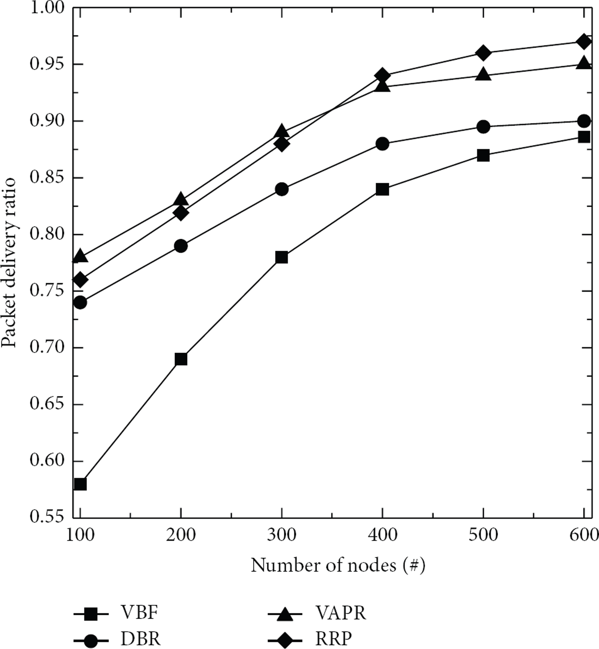
Packet delivery ratio versus number of nodes.

And then, we compared the network throughput with the number of nodes in different routing protocols. As shown in Figure 14, the network throughput of four routing protocols is proportional to the number of nodes. When the number of nodes is not more than 300, the network throughput of VAPR is higher than that of RRP. When the number of nodes increases to 400 and above, the network throughput of RRP is higher than that of VAPR. Overall, RRP improves 13.8% of network throughput than that of VBF on average, 6.4% of network throughput than that of DBR on average, and 0.3% of network throughput than that of VAPR on average.

Figure 14

Network throughput versus number of nodes.

Next, we compared the energy consumption with the number of nodes in different routing protocols. As shown in Figure 15, the energy consumption of four routing protocols is proportional to the number of nodes. RRP performs better than other routing protocols in the same circumstances. When the number of nodes improves from 100 to 600, RRP decreases 28.7% of energy consumption than that of VBF on average, 16.1% of energy consumption than that of DBR on average, and 7.7% of energy consumption than that of VAPR on average.

Figure 15

Energy consumption versus number of nodes.

At last, we compared the average end-to-end delay with the number of nodes in different routing protocols. As shown in Figure 16, the average end-to-end delay of four routing protocols is inversely proportional to the number of nodes. The reason is that when the number of nodes increases, the path from the source node to the target node is closer to the optimal path; therefore, the end-to-end delay decreases. Moreover, when the node density is low, the average end-to-end delay decreases rapidly with density. However, when there are more than 400 nodes deployed in the 3D region, the average end-to-end delay decreases slightly under different node densities. Overall, RRP reduces 22.1% of the end-to-end delay than that of VBF on average, 3.6% of the end-to-end delay than that of DBR on average, and 9.9% of the end-to-end delay than that of VAPR on average.

Figure 16

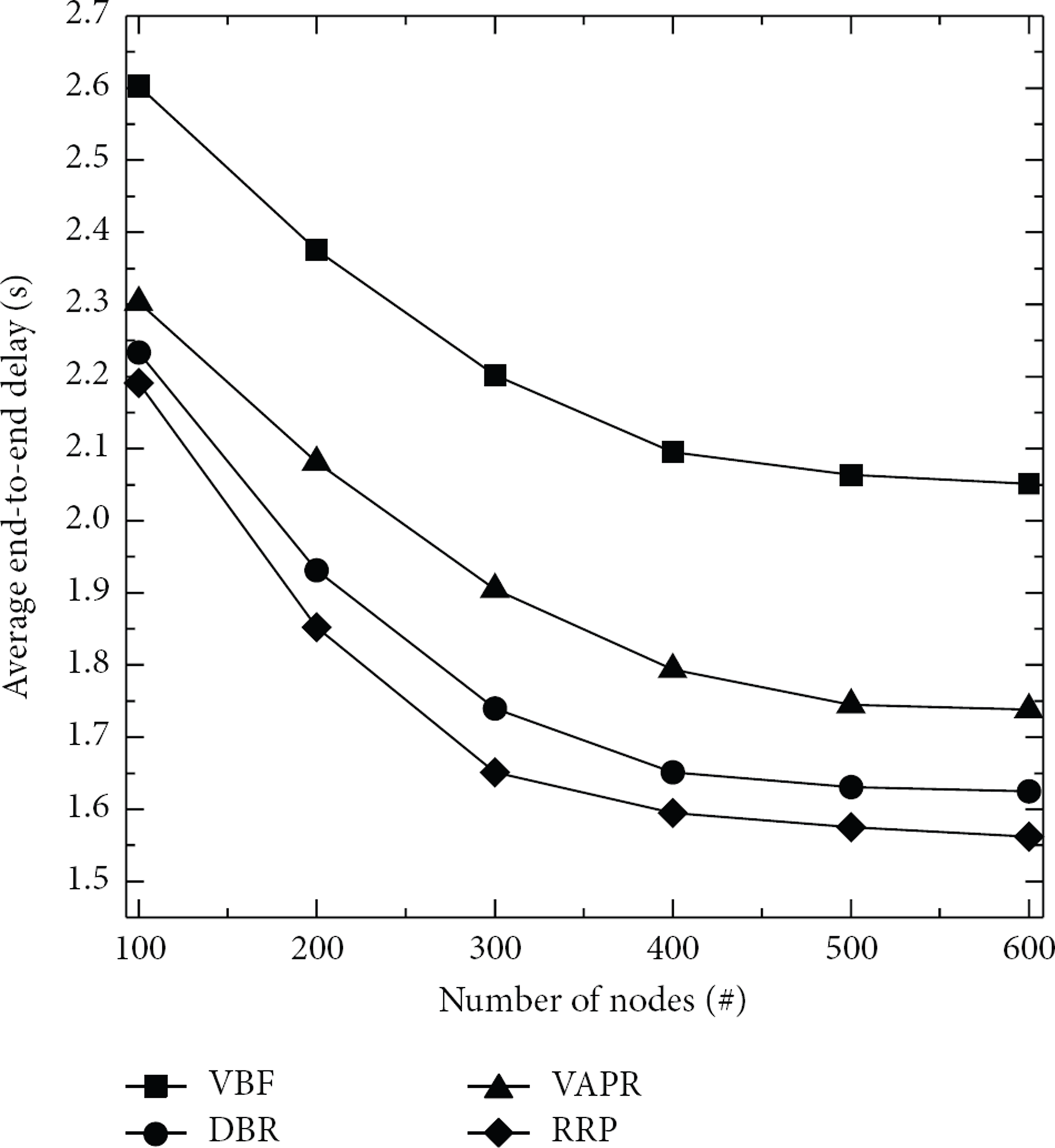
Average end-to-end delay versus number of nodes.

5. Conclusion

In 3D UWSNs, acoustic communication links face high bit error rate, temporary losses, or even permanent failure, which in turn undermine robustness and stability of the routing protocols. In order to deal with the unreliable and unstable nature of the acoustic medium, we have proposed a Robust Routing Protocol for the new features of the 3D UWSNs in order to meet the actual underwater environmental performance needs. RRP is robust against link failure and node failure in that it uses backup links to forward the data packets or enlarges the transmission range to build new links when main routing path is not available. As a result, the routing robustness issue has been well addressed in the proposed route discovery and maintenance processes. Simulation results show that RRP can reduce node failure and link failures' impact in metrics of packet delivery ratio, end-to-end delay, network throughput, and energy consumption.