Coverage Optimization Algorithm Based on Sampling for 3D Underwater Sensor Networks

Abstract

We discuss the problem of maximizing the sensor field coverage for a specific number of sensors while minimizing the distance traveled by the sensor nodes. Thus, we define the movement task as an optimization problem that involves the adjustment of sensor node positions in a coverage optimization mission. We propose a coverage optimization algorithm based on sampling to enhance the coverage of 3D underwater sensor networks. The proposed coverage optimization algorithm is inspired by the simple random sampling in probability theory. The main objective of this study is to lessen computation complexity by dimension reduction, which is composed of two detailed steps. First, the coverage problem in 3D space is converted into a 2D plane for heterogeneous networks via sampling plane in the target 3D space. Second, the optimization in the 2D plane is converted into an optimization in a line segment by using the line sampling method in the sample plane. We establish a quadratic programming mathematical model to optimize the line segment coverage according to the intersection between sensing circles and line segments while minimizing the moving distance of the nodes. The intersection among sensors is decreased to increase the coverage rate, while the effective sensor positions are identified. Simulation results show the effectiveness of the proposed approach.

1. Introduction

A wireless sensor network (WSN) consists of a large number of resource-limited (such as CPU, storage, battery power, and communication bandwidth) tiny devices, which are called sensors. These sensor nodes can sense task specific environmental phenomenon, perform in network processing on the on the sensing field and communicate wirelessly with other sensor nodes or with a sink (also called data gathering node), usually via multihop communications [1]. Water will be the material basis of human sustainable development for affording food, raw materials, and living space for the survival of mankind in the future [2]. However, people cannot easily monitor and develop resources in a large scale because underwater environment is still more serious to human being. Therefore a lot of science and technology communities in different countries have focused on monitoring and exploring underwater resources reasonably by various technologies [3]. Underwater sensor networks are envisioned to enable applications for oceanographic data collection, pollution monitoring, offshore exploration, disaster prevention, assisted navigation, and tactical surveillance applications [4], so it will play an important role in monitoring and developing water resource. The coverage and connectivity are fundamental issues in WSNs, which can determine the scope of services provided by the network, and have a great influence on the network cost and performance of specific applications. The coverage can be considered as a measure of the service quality of WSNs [5, 6].

We analyze the coverage issues in 3D underwater sensor networks (USNs), where sensors are randomly deployed in a 3D field (Figure 1). Underwater sensor nodes are placed in 3D space, and the computational complexity of the coverage optimization algorithm in 3D space is higher than the coverage optimization algorithm in a 2D plane. Therefore, some applications cannot be effectively modeled in 3D space. We propose a 3D coverage optimization algorithm based on sampling (COS) that combines the concepts of simple random sampling in statistics [7] and optimization algorithms [8]. First, we transfer the coverage in 3D space into a 2D plane for heterogeneous networks by plane sampling in a target 3D space. Second, we convert the plane coverage to line segment coverage by the sampling line in the sample plane. Finally, we establish a quadratic programming mathematical model to optimize the line segment coverage according to the intersection between sensing circles and the line segment while minimizing the moving distance of the nodes. The plane coverage should be optimized to enhance the line segment coverage. We summarize the main contributions of our study as follows.

• (1)

  Sample random sampling is applied to the coverage problem in 3D space for dimension reduction.

• (2)

  A quadratic programming mathematical model is established according to the intersection position of the sensing circles and sample line, position of the sensing circles, and radii of the sensing circles.

• (3)

  We conclude that the sum of the node traveling distance for the unchanging node sequence is less than the sum of the changing node sequence. This conclusion is mathematically proven in this study.

• (4)

  A nonlinear quadratic optimization problem is converted into a linear quadratic optimization problem by tightening constraints to obtain the suboptimum solution.

Figure 1

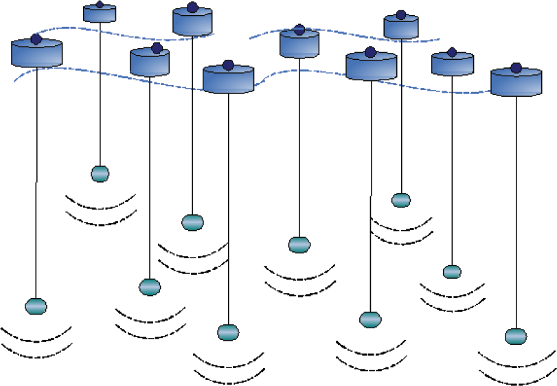
Underwater sensor networks.

The remainder of this paper is organized as follows: Section 2 reviews prior studies on sensor network coverage and discusses related works. Section 3 provides some assumptions and key definitions and describes the system model for underwater wireless sensor networks. Section 4 discusses the development of the mathematical model for sensor network coverage and presents the COS algorithm in detail. Section 5 presents the simulation results of the COS algorithm. Finally, Section 6 concludes and outlines the direction of future works.

2. Related Works

The sensor coverage problem has been extensively studied in the field of multirobot systems and computational geometry the Art Gallery Problem (AGP) and the circumference coverage are related to the coverage of WSNs closely [9]. k-Coverage of sensor networks is one of research focuses in WSNs [1, 10–14]. Huang et al. present a polynomial time algorithm formulating circumference k coverage to a decision problem, whose goal is to determine whether every point in the service area of the sensor network is covered by at least k sensors [10] the optimal deployment density bound for two-coverage deployment patterns is derived in [11] where Voronoi polygons generated by sensor nodes are congruent. The authors design a set of optimal patterns that achieve two-coverage and one-, two-, and three-connectivity thought extending these patterns by considering the connectivity requirement. Ammari and Das focus on coverage and connectivity in 3D WSNs using a continuum percolation theory based approach [13]. The network exhibits a coverage percolation (resp., connectivity percolation) when a giant covered region (resp., giant connected component) almost surely spans the entire network for the first time. It proposes an integrated-concentric-sphere model to address coverage and connectivity in 3D WSNs in an integrated way. Ammari uses Helly's Theorem and the Reuleaux tetrahedron model for characterizing k-coverage of a 3D deployment field and develops a placement strategy of sensors to fully k-cover a 3D field [12, 13].

Coverage algorithm based on virtual force is one of research hotspots currently [15–19]. For a given number of sensors, the VFA algorithm attempts to maximize the sensor field coverage. The sensor nodes are assumed to be deployed in virtual force field; moreover, a judicious combination of attractive and repulsive forces is used to determine virtual motion paths and the rate of movement for the randomly placed sensors. Once the effective sensor positions are identified, a one-time movement with energy consideration incorporated is carried out; that is, the sensors are redeployed to these positions. In [18], Delaunay triangulation is formed with these nodes, and adjacent relationship is defined if two nodes are connected in the Delaunay diagram. Force can only be exerted from those adjacent nodes within the communication range.

The application of linear programming in coverage problem focuses on point (or target) coverage, where the objective is to cover a set of points (targets) [6, 8, 20–22]. Zhao and Gurusamy consider the connected target coverage (CTC) problem with the objective of maximizing the network lifetime by scheduling sensors into multiple sets, each of which can maintain both target coverage and connectivity. The authors determine an upper bound and a lower bound on the network lifetime for the MCT problem and then develops an approximation algorithm to solve it [20]. In [21], the sensing task of covering maximum number of targets while minimizing the energy consumption of the sensing operation is defined as an optimization problem of adjusting the sensing range parameter jointly with selection of nodes in a target coverage mission. A distributed greedy-based heuristic is proposed that nodes with less priority reduce their sensing range before their neighbors and optimal adjustment of sensing range of active nodes is done via a dual-based algorithm. Cardei et al. model the solution as the maximum set covers problem and design two heuristics that efficiently compute the sets, using linear programming and a greedy approach [8]. In [22] the sensor node deployment task has been formulated as a constrained multiobjective optimization problem where the aim is to find a deployed sensor node arrangement to maximize the area of coverage, minimize the net energy consumption, maximize the network lifetime, and minimize the number of deployed sensor nodes while maintaining connectivity between each sensor node and the sink node for proper data transmission.

As described earlier, almost all of coverage strategies in 3D space are based on a premise that sensor nodes are deployed in a specified location and stay there so that the maximum coverage of 3D space is achieved. However, sensor nodes are usually deployed at random and are impossible suspended at specified location without any connection in water. Most of the researches on coverage and connectivity in WSNs are not suitable for underwater because of two-dimensional application only. We propose a 3D coverage optimization algorithm for underwater 3D sensor networks (USNs) in which sensor nodes are randomly deployed and are fixed by cables, in which quadratic programming is applied to coverage optimization problem in 2D plane and 3D space.

3. Assumptions and Definitions

3.1. Assumptions

We assume that a large number of underwater sensors are distributed in an area of interest. A 3D USN model is described as follows [23, 24].

• (1)

  A 3D USN contains two types of sensor nodes: one is used for communications and is deployed on the water surface; the other is used for sensing and is deployed underwater.

• (2)

  All sensor nodes that are deployed underwater have homogeneous models; that is, all sensors have binary sensing coverage models. Thus, the sensing model is a sphere, and all sensors adopt the radius R of the sensing sphere model.

• (3)

  The underwater sensor node communicates with the surface node via a cable that connects the two sensors.

• (4)

  Sensor node position and depth can be acquired via the sensor nodes deployed on the water surface and cables.

• (5)

  The sensor nodes on the water surface are fixed in place with an anchor. However, the underwater nodes can move to a specified location vertically.

• (6)

  Sensor nodes have enough residual energy to move the specified location because coverage algorithm is executed during network initialization.

We assume that sensor nodes are randomly deployed in a 3D cuboid space and denote the distance between two spots as a Euclidean distance.

3.2. Definitions

Definition 1 (binary sensor model).

Suppose that the distance between sensor node $X_i$ and space spot Y is $D(X_i,Y)$ and that each sensor node has a sensing range R. The sensing probability is shown as follows:

$$\begin{array}{cc}& p\left(X_i,Y\right)=\{\begin{array}{cc}\mathrm{1}\hfill & D\left(X_i,Y\right)<R,\hfill \\ \mathrm{0}\hfill & \text{else}.\hfill \end{array}\end{array}$$

(1)

Definition 2 (sensing sphere).

Sensor node $X_i$ is positioned at $(x_i,y_i,z_i)$ , and the sensor model is the binary sensor model with radius R. Thus, the coverage space of the sensor node underwater is a sphere with a center located at $(x_i,y_i,z_i)$ . The radius is denoted by R.

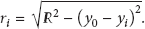
Definition 3 (sensing circle).

The distance of underwater sensor node $X_i$ to the sample plane H is $d_i\hspace{0.17em}\hspace{0.17em}(d_i<R)$ . When the sensing sphere of $X_i$ and sample plane H intersect, a circle in the plane will be formed. The circle center is the projection of $X_i$ to H, and the radius of the circle is $\sqrt{R^{\mathrm{2}}-d_i^{\mathrm{2}}}$ .

Definition 4 (sample plane).

An arbritrary plane in 3D space intersect the boundary of 3D monitoring space to form polygon MNOP, as shown in Figure 2. The plane area which is contained by polygon MNOP is defined as sample plane.

Figure 2

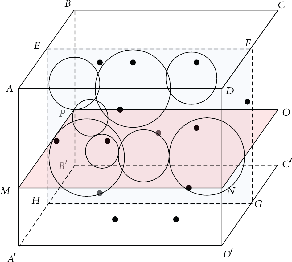
Coverage model in underwater 3D space.

Definition 5 (sample line).

Choose a line at random in sample plane and denote it as “c”, line c, and the boundary of sample plane intersect at points A and B, as illustrated in Figure 3. Line $AB$ is defined as sample line.

Figure 3

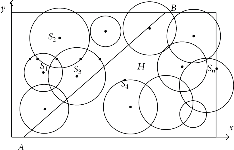
Sampling line.

Definition 6 (coverage rate).

Coverage rate η is determined by the ratio between the volume of coverage space P and the volume of deployed space S, which is given by the following equation:

$$\begin{array}{cc}& \eta =\frac{V_P}{V_S}.\end{array}$$

(2)

3.3. Problem Definition

The proposed algorithm attempts to maximize the coverage of USNs while striving to minimize the movement distance of the nodes. This problem can be defined as follows: given that n sensors are randomly and uniformly deployed on the surface of the ocean/sea, we devise an algorithm that maximizes the total 3D coverage of the nodes and minimizes the message and travel distance complexity. As mentioned in the Introduction, we seek a fully distributed algorithm that will enable the sensor nodes to self-organize before data collection commences. Our proposed algorithm has five phases: (1) sample plane in a target 3D space, (2) sample line in the sample plane, (3) establishment of a quadratic programming mathematical model to optimize line segment coverage, (4) depth assignment, and (5) additional rounds.

4. Coverage Optimization Algorithm Based on Sampling

The sample planes intersect with the sensing spheres. The distance of the center of the sensing spheres to the sample planes is less than R. The intersection of the sensing spheres and sample planes are a set of sensing circles with different radii (Figure 4). We analyze the influence of the position of coverage circles on the coverage rate of sample planes in the $x\text{-}y$ and $x\text{-}z$ directions. Although sensor nodes move in the z-axis, the radii of the sensing circles will change in the horizontal plane and locations will remain unchanged, respectively. In the vertical plane, the sensing circles also move in the z-axis; however, the radii of these sensing circles contain an original value. A coverage optimization algorithm is executed to change the radii and locations of the sensing circles in the sample planes. Thereafter, the sensor nodes corresponding to the sensing circles will be redeployed according to the new radii and locations of the sensing circles.

Figure 4

Sensing circle.

4.1. Coverage Optimization Analysis Based on the Horizontal Sample Plane

$MNOP$ is a horizontal sample plane in 3D space and has a plane function of $z=z_{\mathrm{0}}$ (Figure 4). The sample plane interacts with the coverage sphere to form a coverage circle (Figure 5). The radius of the sample plane is expressed as follows:

$$\begin{array}{cc}& r_i=\sqrt{R^{\mathrm{2}}-{\left(z_i-z_{\mathrm{0}}\right)}^{\mathrm{2}}}.\end{array}$$

(3)

Figure 5

Sensing circles in a horizontal sample plane.

$AB$ is a random straight line in plane $MNOP$ . The distance of lines $A_l{B}_l$ and $A_h{B}_h$ to line $AB$ is R. Suppose that n sensing circles exists $(S_{\mathrm{1}},S_{\mathrm{2}},\dots ,S_n)$ and that the centers of these sensing circles are located between lines $A_l{B}_l$ and $A_h{B}_h$ . Each of these sensing circles may intersect with line $AB$ ; for example, $S_i$ and line $AB$ may intersect at points $(x_{il},y_{\mathrm{0}})$ and $(x_{ih},y_{\mathrm{0}})$ . We describe the sensing line segment of line $AB$ and $S_i$ as a set; that is, $C_i=\{x/x_{il}\le x\le x_{ih}\}$ . $C_i$ will be an empty set if $S_i$ and line $AB$ do not intersect. The union of these sets should include line segment set $C=\{x/\mathrm{0}\le x\le l\}$ , and straight line $AB$ is completely covered by the sensing circles

$$\begin{array}{cc}& {\displaystyle \bigcup }_{i=\mathrm{1}}^n{C}_i\supset C.\end{array}$$

(4)

The radii of the sensing circles increase as the underwater sensor node moves closer to plane $EFGH$ in the z-axis. Thus, the sensing line segment is longer than the previous sensing line segment. The radius of the sensing circle corresponding to the underwater sensor node increases with the movement of the underwater sensor node toward the plane.

Suppose that the center of the ith sensing circle is at $(x_i,y_i)$ and that the radius is $r_i$ . For $r_i+\mathrm{\Delta }{r}_i>|y_i-y_{\mathrm{0}}|$ , the sensing circle intersects line $AB$ . The points of the intersection are shown as follows:

$$\begin{array}{cc}& x_{il}=x_i-\sqrt{{\left(r_i+\mathrm{\Delta }{r}_i\right)}^{\mathrm{2}}-y_i^{\mathrm{2}}},\end{array}$$

(5)

$$\begin{array}{cc}& x_{ih}=x_i+\sqrt{{\left(r_i+\mathrm{\Delta }{r}_i\right)}^{\mathrm{2}}-y_i^{\mathrm{2}}}.\end{array}$$

(6)

For $R_i+\mathrm{\Delta }{R}_i<y_i$ , the segment set corresponding to the sensing circle will be empty because the sensing circle and line $AB$ do not intersect. This problem is hard to resolve because of two reasons: the constraints in (5) cannot be algebraically described because confirming the relationship among the sets $(C_{\mathrm{1}},C_{\mathrm{2}},\dots ,C_n,C)$ is difficult; this problem is a nonlinear programming problem because the upper and lower bounds of the sets and variables $(\mathrm{\Delta }{R}_{\mathrm{1}},\mathrm{\Delta }{R}_{\mathrm{2}},\dots ,\mathrm{\Delta }{R}_n)$ are nonlinear, so the problem is hard to be resolved [21].

4.2. Coverage Optimization Analysis Based on the Vertical Sample Plane

In this section, we derive the optimization coverage in a vertical sample plane (Figures 6 and 7). $EFGH$ is a vertical sample plane, and the function of plane $EFGH$ is $y=y_0$ . $MN$ is a random straight line in plane $EFGH$ and is parallel to the z-axis. Line $MN$ intersects n sensing circles $(S_1,S_2,\dots ,S_n)$ , which correspond to n sensor nodes $(X_1,X_2,\dots ,X_n)$ . The sensor nodes $(X_1,X_2,\dots ,X_n)$ are located at $(x_1,y_1,z_1),(x_2,y_2,z_2),\dots ,(x_n,y_n,z_n)$ , and the centers of the sensing circle are located at $(x_1,z_1)$ , $(x_2,z_2),\dots ,(x_n,z_n)$ . Plane $EFGH$ has $z_1\le z_2\le \cdots \le z_n$ . The radii of the sensing circles are expressed as follows:

$$\begin{array}{cc}& r_i=\sqrt{R^{\mathrm{2}}-{\left(y_{\mathrm{0}}-y_i\right)}^{\mathrm{2}}}.\end{array}$$

(7)

Figure 6

Vertical sample plane in underwater 3D space.

Figure 7

Vertical sample plane.

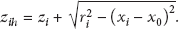
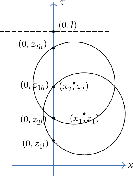
Definition 7 (upper and lower intersections).

Coverage circle $S_i$ and sample line ( $x=x_0$ ) intersect at points $(x_0,z_{il})$ and $(x_0,z_{ih})$ , where $z_{il}<z_{ih}$ . Points $(x_0,z_{il})$ and $(x_0,z_{ih})$ are denoted as the upper lower intersections, respectively, (Figure 8).

Figure 8

Upper and lower intersection points.

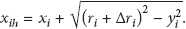
The sensing circles and line segments intersect at $(x_0,z_{1l})$ , $(x_0,z_{1h}),(x_0,z_{2l})$ , $(x_0,z_{2h}),\dots ,(x_0,z_{nl})$ , $(x_0,z_{nh})$ . The intersection segments of the sensing circles and line $MN$ are described as sets; that is, $Z_1=\{z/z_{1l}\le z\le z_{1h}\},Z_2=\{z/z_{2l}\le z\le z_{2h}\},\dots ,Z_n=\{z/z_{nl}\le z\le z_{nh}\}$ . The union of these segment sets should include the segment set $Z=\{z/0\le z\le h\}$ if line $MN$ is completely covered by sensing circles

$$\begin{array}{cc}& {\displaystyle \bigcup }_{i=\mathrm{1}}^n{Z}_i\supset Z,\end{array}$$

(8)

$$\begin{array}{cc}& z_{il}=z_i-\sqrt{r_i^2-{\left(x_i-x_0\right)}^2},\end{array}$$

(9)

$$\begin{array}{cc}& z_{ih}=z_i+\sqrt{r_i^2-{\left(x_i-x_0\right)}^2}.\end{array}$$

(10)

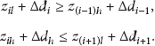
The sensing line segments move with the corresponding underwater sensor nodes moving in z-axis, but the length of sensing line segment is unchanged. We suppose that the movement distance of n sensing circles is $\mathrm{\Delta }{d}_1,\mathrm{\Delta }{d}_2,\dots ,\mathrm{\Delta }{d}_n$ separately. The sensing line segments after moving are described by sets, that is, $(z_{1l}+\mathrm{\Delta }{d}_1,z_{1h}+\mathrm{\Delta }{d}_1),(z_{2l}+\mathrm{\Delta }{d}_2,z_{2h}+\mathrm{\Delta }{d}_2),\dots ,(z_{nl}+\mathrm{\Delta }{d}_n,z_{nh}+\mathrm{\Delta }{d}_n)$ . The optimization algorithm is developed to deal with the sample straight line coverage completely with the object minimum of the sum of sensing line segment moving distance. That is,

$$\begin{array}{cc}& \begin{array}{cc}\min \hfill & {\displaystyle \sum }_{i=\mathrm{1}}^n\mathrm{\Delta }{d}_i^{\mathrm{2}}\hfill \\ \text{st:}\hfill & {\displaystyle \bigcup }_{i=\mathrm{1}}^n(z_{il}+\mathrm{\Delta }{d}_i,z_{ih}+\mathrm{\Delta }{d}_i)\supset \left(\mathrm{0},h\right).\hfill \end{array}\end{array}$$

(11)

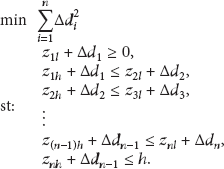
Constraint conditions are shown as

$$\begin{array}{l}\min (z_{1l}+\mathrm{\Delta }{d}_1,z_{2l}+\mathrm{\Delta }{d}_2,\dots ,z_{nl}+\mathrm{\Delta }{d}_n)<\mathrm{0},\\ z_{2l}+\mathrm{\Delta }{d}_2>z_{1h}+\mathrm{\Delta }{d}_1,\\ z_{3l}+\mathrm{\Delta }{d}_3>\max \left(z_{1h}+\mathrm{\Delta }{d}_1,z_{2h}+\mathrm{\Delta }{d}_2\right),\\ \phantom{z_{3l}+\mathrm{\Delta }{d}_3>\max }⋮\\ z_{nl}+\mathrm{\Delta }{d}_n>\max \left(z_{1h}+\mathrm{\Delta }{d}_1,z_{2h}+\mathrm{\Delta }{d}_2,\dots ,z_{\left(n-1\right)h}+\mathrm{\Delta }{d}_{n-1}\right),\\ \max \left(z_{1h}+\mathrm{\Delta }{d}_1,z_{2h}+\mathrm{\Delta }{d}_2,\dots ,z_{nh}+\mathrm{\Delta }{d}_n\right)>h.\end{array}$$

(12)

It is difficult to find the optimal solution because the previous problem is nonlinear. Therefore we seek the feasible solution by tightening constraints. First, we analyze the affection of the sensing circles’ position on optimization algorithm.

Theorem 8.

The sum of the traveled distance of the nodes is small when the order of the nodes remains the same compared with other nodes.

Proof.

We assume that only two sensing circles $S_1,S_2$ with centers located at $(x_1,z_1)$ and $(x_2,z_2)$ exist in interval $(\mathrm{0},l)$ (Figure 9). Suppose that $z_1<z_2$ . These two sensing circles and the z-axis intersect at points $(0,z_{1l})$ , $(\mathrm{0},z_{1h})$ and $(0,z_{2l})$ , $(\mathrm{0},z_{2h})$ . The spot coordinates are expressed as follows:

$$\begin{array}{cc}& z_{1h}-z_{1l}+z_{2h}-z_{2l}>l,\\ 0\le z_{1l},z_{1h},z_{2l},z_{2h}\le l.\end{array}$$

(13)

Both $\mathrm{\Delta }{d}_1$ and $\mathrm{\Delta }{d}_2$ are the moving distance of sensing circles $S_1$ and $S_2$ , respectively. We assume that both sensing circles will be arranged in the same order along the z-axis after optimization coverage

$$\begin{array}{cc}& z_{\mathrm{1}}+\mathrm{\Delta }{d}_{\mathrm{1}}<z_{\mathrm{2}}+\mathrm{\Delta }{d}_{\mathrm{2}}.\end{array}$$

(14)

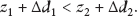
The complete coverage of line segment $(0,l)$ implies the following:

$$\begin{array}{cc}& z_{2h}+\mathrm{\Delta }{d}_2\ge l,\\ z_{1l}+\mathrm{\Delta }{d}_1\le 0.\end{array}$$

(15)

We then derive the following equation:

$$\begin{array}{cc}& \left|\mathrm{\Delta }{d}_{\mathrm{1}}\right|+\left|\mathrm{\Delta }{d}_{\mathrm{2}}\right|\ge l-z_{\mathrm{2}h}+z_{\mathrm{1}l}.\end{array}$$

(16)

The minimum moving distance of the sensing circles is computed as follows:

$$\begin{array}{cc}& \mathrm{\Delta }{d}_{\min }=l-z_{\mathrm{2}h}+z_{\mathrm{1}l}.\end{array}$$

(17)

We obtain $z_1+\mathrm{\Delta }{d}_1>z_2+\mathrm{\Delta }{d}_2$ , and the order of the sensing circles changes. The complete coverage of line segment $(0,l)$ implies the following:

$$\begin{array}{cc}& z_{1h}+\mathrm{\Delta }{d}_1^{\prime }\ge l,\\ z_{2l}+\mathrm{\Delta }{d}_2^{\prime }\le 0.\end{array}$$

(18)

Equations (18) denote the following:

$$\begin{array}{cc}& \left|\mathrm{\Delta }{d}_{\mathrm{1}}^{\prime }\right|+\left|\mathrm{\Delta }{d}_{\mathrm{2}}^{\prime }\right|\ge l-z_{\mathrm{1}h}+z_{\mathrm{2}l}.\end{array}$$

(19)

Thus, the minimum moving distance of the sensing circles is computed as follows:

$$\begin{array}{cc}& \mathrm{\Delta }{d}_{\min }^{\prime }=l-z_{\mathrm{1}h}+z_{\mathrm{2}l};\end{array}$$

(20)

that is,

$$\begin{array}{cc}& \mathrm{\Delta }{d}_{\min }^{\prime }-\mathrm{\Delta }{d}_{\min }=z_{\mathrm{2}h}+z_{\mathrm{2}l}-z_{\mathrm{1}h}-z_{\mathrm{1}l}.\end{array}$$

(21)

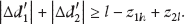
According to the nature of the circle, we derive the following equation:

$$\begin{array}{cc}& z_{\mathrm{2}}=\frac{z_{\mathrm{2}l}+z_{\mathrm{2}h}}{\mathrm{2}}\ge z_{\mathrm{1}}=\frac{z_{\mathrm{1}l}+z_{\mathrm{1}h}}{\mathrm{2}}.\end{array}$$

(22)

Thus, $z_{2l}+z_{2h}-z_{1l}-z_{1h}\ge 0$ ; that is, $\mathrm{\Delta }{d}_{\min }^{\prime }>\mathrm{\Delta }{d}_{\min }$ . We conclude that the sum of the moving distance of sensing circles in the same order is less than the sum of the moving distance of sensing circles in different orders. Thus, n sensing circles intersect at the sampling line and can be decomposed into multicoupled combinations of mobile nodes. After executing the coverage optimization algorithm, each pair of sensing circles will maintain their order. Thus, the order of all nodes will not change.

Figure 9

Position of two sensing circles.

On the basis of the previous analysis, we assume that the relative order of the sensing circles after optimization is the same before optimization. We propose different constraint conditions depending on the length of the sensing line segments. The length of the sensing line segment is $z_{ih}-z_{il}$ , and the sensing circle $S_i$ and sample line intersect at $(x_0,z_{il})$ and $(x_0,z_{ih})$ . If n sensing circles intersect at the sample straight line, the sum of the length of the sensing line segments can be written as follows:

$$\begin{array}{cc}& L={\displaystyle \sum }_{i=\mathrm{1}}^n(z_{ih}-z_{il}).\end{array}$$

(23)

For $L\ge h$ , the sample can be completely covered by sensing circles. Therefore, the intersection coordinates of the sensing circle $S_i$ and straight line imply the following inequalities:

$$\begin{array}{cc}& z_{il}+\mathrm{\Delta }{d}_i\ge z_{\left(i-1\right)h}+\mathrm{\Delta }{d}_{i-1},\\ z_{ih}+\mathrm{\Delta }{d}_h\le z_{\left(i+1\right)l}+\mathrm{\Delta }{d}_{i+1}.\end{array}$$

(24)

The upper intersection of circle $S_i$ should be the lower side of the lower intersection of sensing circle $S_{i-1}$ . The lower intersection of circle $S_i$ should be the upper side of the upper intersection of sensing circle $S_{i+1}$ . The constraint conditions of the optimization algorithm follow the following equation:

$$\begin{array}{cc}& \begin{array}{cc}\min \hfill & {\displaystyle \sum }_{i=\mathrm{1}}^n\mathrm{\Delta }{d}_i^{\mathrm{2}}\hfill \\ \text{st:}\hfill & \begin{array}{c}{z}_{\mathrm{1}l}+\mathrm{\Delta }{d}_{\mathrm{1}}\le \mathrm{0},\\ z_{\mathrm{2}l}+\mathrm{\Delta }{d}_{\mathrm{2}}\ge z_{\mathrm{1}h}+\mathrm{\Delta }{d}_{\mathrm{1}},\\ z_{\mathrm{3}l}+\mathrm{\Delta }{d}_{\mathrm{3}}\ge z_{\mathrm{2}h}+\mathrm{\Delta }{d}_{\mathrm{2}},\\ ⋮\\ z_{nl}+\mathrm{\Delta }{d}_n\ge z_{\left(n-\mathrm{1}\right)h}+\mathrm{\Delta }{d}_{n-\mathrm{1}},\\ z_{nh}+\mathrm{\Delta }{d}_n\ge h.\end{array}\hfill \end{array}\end{array}$$

(25)

For $L<h$ , the sample cannot be considered a solution to the optimization problem because the sample straight line cannot be fully covered by sensing circles. Therefore, the maximum coverage of the sample straight line is expected. The sample straight line is covered maximally when the sensing line segments in the sample straight line are disjointed. We establish the new optimization algorithm as follows:

$$\begin{array}{cc}& \begin{array}{cc}\min \hfill & {\displaystyle \sum }_{i=\mathrm{1}}^n\mathrm{\Delta }{d}_i^{\mathrm{2}}\hfill \\ \text{st:}\hfill & \begin{array}{c}{z}_{\mathrm{1}l}+\mathrm{\Delta }{d}_{\mathrm{1}}\ge \mathrm{0},\\ z_{\mathrm{1}h}+\mathrm{\Delta }{d}_{\mathrm{1}}\le z_{\mathrm{2}l}+\mathrm{\Delta }{d}_{\mathrm{2}},\\ z_{\mathrm{2}h}+\mathrm{\Delta }{d}_{\mathrm{2}}\le z_{\mathrm{3}l}+\mathrm{\Delta }{d}_{\mathrm{3}},\\ ⋮\\ z_{(n-\mathrm{1})h}+\mathrm{\Delta }{d}_{n-\mathrm{1}}\le z_{nl}+\mathrm{\Delta }{d}_n,\\ z_{nh}+\mathrm{\Delta }{d}_{n-\mathrm{1}}\le h.\end{array}\hfill \end{array}\end{array}$$

(26)

The new positions of the sensing circles are $(x_1,z_1+\mathrm{\Delta }{d}_1)$ , $(x_2,z_2+\mathrm{\Delta }{d}_2),\dots ,(x_n,z_n+\mathrm{\Delta }{d}_n)$ , and the corresponding sensor nodes are located at $(x_1,y_1,z_1+\mathrm{\Delta }{d}_1)$ , $(x_2,y_2,z_2+\mathrm{\Delta }{d}_2),\dots ,(x_n,y_n,z_n+\mathrm{\Delta }{d}_n)$ . Figures 10(a) and 10(b) illustrate the position of the sensing circles after random placement and the final sensor positions determined by the COS algorithm, respectively. Figures 10(a) and 10(b) illustrate an example of $L\ge h$ , whereas Figures 11(a) and 11(b) illustrate an example of $L<h$ .

Figure 10

$L\ge W$ example.

Figure 11

$L<W$ example.

We find a feasible solution after limiting the constraints of the optimization algorithm in vertical planes. Moreover, the 2D plane coverage optimization in the y-z direction is similar to the x-z direction. Thus, we only sample the vertical plane in underwater 3D space (Figure 6).

4.3. Complete Algorithm

The pseudocode of the COS algorithm and the single sample plane coverage function are presented in Algorithms 1 and 2, and the flowchart of the single sample line coverage function is presented in Figure 12. The following parameters are defined for the mathematical modeling process:

•  

  Sensor_set: the set of sensor node position, $S_i\hspace{0.17em}\hspace{0.17em}(x_i,y_i,z_i)\in$   Sensor_set,

•  

  circle_set: the set of sensing circle position and radius,

•  

  circle_N_set: the set of sensing circle position and radius after optimization,

•  

  d_step_plane: the step size of plane sampling,

•  

  d_step_line: the step size of line sampling,

•  

  (l, w, h): the length, width, and height of the 3D space, respectively,

•  

  x_int, y_int: the initial position of the sample line in the x and y directions, respectively,

•  

  x_line, y_line: the position of the sample line in the x and y directions, respectively,

•  

  R: the sensing radius of the sensor node.

Algorithm 1: Pseudocodes for the COS algorithm.

COS algorithm

%Input: Sensor_set, d_step_plane, d_step_line, l, w, h, x_int, y_int, R

%Output: Sensor_set.

Main procedure:

(1)     $y=\text{random}(\mathit{0},R/\mathit{2})$ ; % the initial position of sample plane in $x-z$ .

(2)   While $y<l$

(3)  For $S_i\left(x_i,y_i,z_i\right)$ ∈Sensor_set

(4)   If (the sensing sphere and sample plane intersect)

(5)    calculate the radius of the sensing circle according to (7), and save the position $\left(x_i,z_i\right)$ and radius $r_i$ of sensing circle

     to circle_set.

(6)   End

(7)  end

(8)  circle_N_set = plane_cover(circle_set, x_int, w, h, d_step_line);

      % the single sample plane coverage optimization function and its procedure are shown in Figure 11.

(9)  Update the position set Sensor_set according to circle_N_set.

(10)       $y=y+d$ _step_plane

(11)      Empty the set circle_set, circle_N_set;

(12) End

(13)  $x=\text{random}(\mathit{0},R/\mathit{2})$ ; % initial position of the sample plane in $y-z$ .

(14) While $x<w$

(15)      For $S_i$ ∈Sensor_set

(16)       If (the sensing sphere and sample plane intersect)

(17)        calculate the radius of the sensing circle according to (7), and save the position $\left(x_i,z_i\right)$ and radius $r_i$ of the sensing

     circle to circle_set.

(18)       End

(19)      end

(20)     circle_N_set = plane_cover(circle_set,y_int, l, h, d_step_line);

(21)      Update the position set Sensor_set according to circle_N_set;

(22)      $x=x+d$ _step_plane;

(23)     Empty the set circle_set, circle_N_set;

(24)     End

Algorithm 2: Pseudocodes for plane coverage.

Plane coverage

function circle_N_set = plane_cover(circle_set, x_int,

$w,h,d$ _step_line)

(1) x_line = x_int;

(2) while x_line < w

(3)  circle_N_set = line_cover(circle_set, x_line, h);

  % the sample line coverage optimization function

  and its flowchart is shown in Figure 12;

(4)  x_line = x_line + d;

(5)  circle_set = circle_N_set;

(6) end

Figure 12

Straight line coverage flowchart.

The COS algorithm is performed by the sink node on land. First, a plane that is parallel to the x-z plane is sampled in interval (0, $R/2$ ) (Line 1). In Lines 3 to 6 of the COS algorithm, the positions and radii of the sensing circles in the sampling plane are calculated if the sensing spheres intersect at the sampling plane. The plane coverage subroutine is invoked in Line 8 to optimize the sampling plane coverage. Thereafter, the sink node sends DEPTH messages to the underwater sensor nodes. Any node receiving a DEPTH message performs its specified movement (Line 9). After the first optimization, additional planes are sampled according to the step length until the sampling plane is beyond the boundary of 3D space, and the optimization algorithm is conducted numerously to optimize all sampling planes coverage. Additional rounds are also conducted when the sampling planes are parallel to the y-z plane to increase the total coverage in Lines 14–24.

Given the sampling plane function, the position of the initial sampling line, boundary of the plane, step length of the sampling, and positions and radii of the sensing circles, the subprogress can be used to optimize the coverage of the sampling plane. Line 1 is the line function of the initial sampling line. Line 3 performs the line coverage optimization function and calculates the new positions of the sensing circles. Additional optimization sequences are conducted until the sampling line is beyond the boundary of the sampling plane.

We describe the single-line coverage optimization function in a flowchart (Figure 12). The following equation is the expression of single-line coverage optimization function:

$$\begin{array}{cc}& \text{function}\hspace{0.17em}\text{circle\_}N\text{\_set}=\text{line\_cover}\hspace{0.17em}(\text{circle\_set},x\_\text{line},h).\end{array}$$

(27)

5. Simulation

In this section, we describe the simulation setup, performance metrics, and performance results of the study. We assume that all messages can be transmitted/received without any errors and that the sensor nodes are uniformly distributed in a 100 m × 100 m × 100 m 3D space. The sensing radius of the underwater sensor node is 20 m, and the communication nodes that are deployed on the water surface can communicate with each other. A coordinator node is attached to the server and acts as a gateway to the USNs. The server implements the COS algorithm presented in Section 4 and conveys the new position of the underwater sensor nodes to the coordinator. The location of an underwater sensor node is adjusted by its corresponding buoy via the cable after receiving the information.

Figure 13 shows the initial position of the sensing circles in one of the vertical sample planes after random distribution. Figure 14 shows the final position of the sensing circles of the COS algorithm in the same vertical sample planes. We observe that the overlap area in Figure 14 is less than the overlap area in Figure 13.

Figure 13

Initial position of the sensing circles after random distribution.

Figure 14

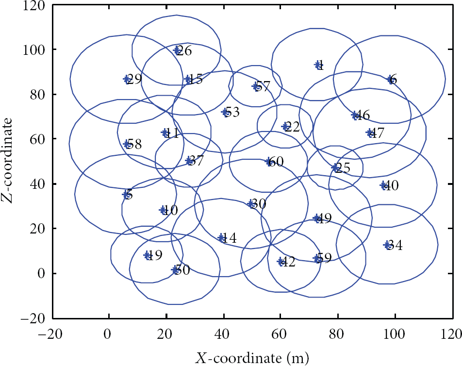
Position of the sensing circles after execution of the COS algorithm.

Figure 15 shows the coverage rate comparison between the random placement and COS algorithm in the sample vertical planes. The simulation is conducted with 60 sensor nodes, and the sensing range is set to 20 m. The sampling plane coverage rate of the COS algorithm outperforms the random approach by approximately 10%. This improvement is insignificant and is caused by the limited movement direction of the nodes (i.e., vertical movement only).

Figure 15

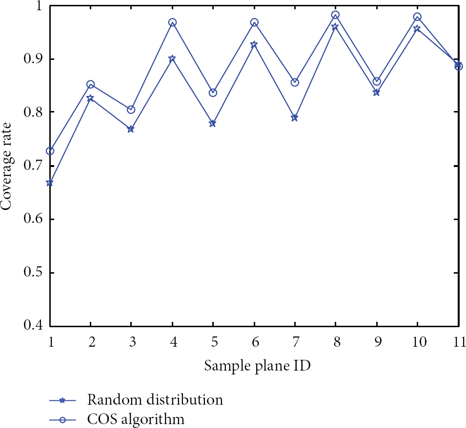
Coverage rate of sample planes for different distributions.

We have conducted experiments with different node quantities. The results shown in Figure 16 clearly reveal that our algorithm is valid for various node quantities. The simulation is implemented twice, and the sensing range is set to 20 m. The COS algorithm outperforms the random approach by approximately 10% in terms of coverage. The performance of the COS algorithm is superior when the number of nodes is relatively few. Considering that the 3D space coverage and node deployment on the surface have a close relationship, the optimal coverage in 3D space will be achieved by the COS algorithm if the nodes on the surface are distributed well.

Figure 16

Coverage rate for the number of nodes.

Figure 17 presents the simulation results in different sampling steps for 40 to 80 underwater sensor nodes. The algorithm performance is weak when additional iterations are implemented because the optimization in the second plane will have a negative effect on the first plane if two adjacent planes intersect at the same sensing sphere.

Figure 17

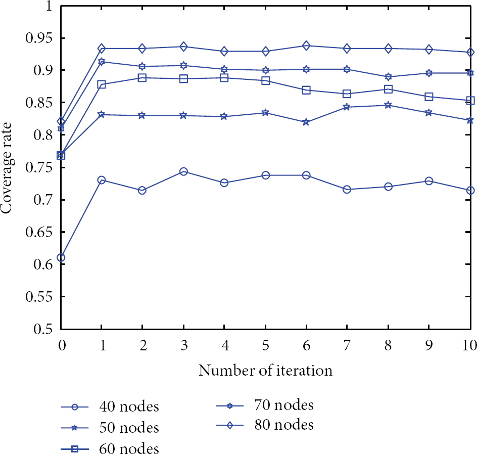
Coverage rate for iterations.

Similarly, when sensing range is increased while the number of nodes is fixed as 60 and 80, respectively, coverage increases as seen in Figures 18 and 19. The patterns show that the coverage can be effectively enhanced by the COS algorithm. We consider the influence of node quantity, iteration, and sensing range in the experiments and find that the proposed algorithm works effectively under extreme surroundings.

Figure 18

Coverage versus the sensing radius for 60 nodes.

Figure 19

Coverage versus sensing radius for 80 nodes.

6. Conclusion

This study proposes a 3D COS to enhance the coverage of USNs. We convert a 3D space coverage into a 2D plane coverage for heterogeneous networks by a sampling plane in the target 3D space. The positions of the sensing circles in the sample plane are calculated by the COS algorithm to enhance coverage. Thereafter, the sensor nodes that correspond to the sensing circles are redeployed. The simulation results show that the COS algorithm can improve the coverage provided by an initial random placement. To a certain degree, the coverage in the 3D space improves when the iterations increase. However, the coverage will remain unchanged or decrease when the number of iterations surpasses a certain value for the adjacent sample planes. The performance of the COS algorithm is affected by two aspects:

• (1)

  for the limitation of the network model, the coverage cannot be significantly improved when the wireless sensor nodes are nonuniformly distributed,

• (2)

  the COS algorithm is performed on each sample plane alone because we do not consider the relativity between the adjacent sample planes.

In the future, we will consider the relativity of the sample planes to ensure the flexibility of the COS algorithm as well as adjust the positions of the wireless sensor nodes on the water surface to distribute uniformly the sensor nodes and enhance their coverage in 3D space.