Sage Journals: Discover world-class research

Abstract

Laminar mixed convection in the entrance region of horizontal and inclined semicircular ducts has been investigated. The governing momentum and energy equations were solved numerically using a marching technique with finite control volume approach following the SIMPLER algorithm. Results were obtained for thermal boundary condition of uniform heat input axially and uniform wall temperature circumferentially, incorporating Pr = 7, Re = 500, inclination angles (α = 0° and 20°), and a wide range of Grashof numbers. These results include velocity and temperature distributions at different axial locations as well as axial distribution of local Nusselt number and local wall friction factor. It was found that Nusselt number is close to the forced convection values near the entrance region, then decreases to minimum value as the distance from the entrance increases, and then rises due to the effect of free convection before reaching a constant value (fully developed). As Grashof number increases Nusselt number and wall friction factor increase in both developing and fully developed regions for horizontal and inclined ducts. A comparison with the experimental data in the thermal entrance region was also conducted and the comparison was satisfactory.

1. Introduction

Laminar combined forced and free convection flows in ducts received much attention in the recent years because of their wide range of applications, such as compact heat exchangers. This paper is concerned with the problem of laminar mixed convection in the entrance region of horizontal and inclined semicircular ducts with axial uniform heating. Due to the large amount of literature on fully developed laminar mixed convection for different cross sections and inclination angles, consideration will be given to the geometry of semicircular ducts only. Nandakumar et al. [1] studied numerically the problem of fully developed laminar mixed convection flow in horizontal semicircular ducts for the H1 thermal boundary condition with the flat wall at the bottom. Lei and Trupp [2] solved the same problem considered in [1] with the flat wall on top. They reported approximately the same results of Nusselt number as for the flat wall at the bottom [1]. Chinproncharoepong et al. [3] studied the effect of orientation by rotating the horizontal semicircular duct from 0° (the flat wall on top) to 180° (the flat wall at the bottom) with incremental angle of 45°. Busedra and Soliman [4] investigated the effect of duct inclination on laminar mixed convection in inclined semicircular ducts under buoyancy-assisted and opposed conditions. They oriented the flat wall of the duct in vertical position using two thermal boundary conditions H1 and H2; H2 thermal boundary condition is defined as a constant heat flux axially and circumferentially.

The literature on combined free and forced convection in the entrance region is few in comparison with the fully developed case. Most of the results for laminar mixed convection in the entrance region are available for vertical rectangular ducts [5 –7] and for vertical circular tubes [8, 9]. Other results for horizontal duct are also available for rectangular ducts [10], concentric annulus [11], and circular tubes [12]. The available numerical solution for laminar mixed convection of upward airflow in the entrance region between inclined parallel plates with uniform wall temperature are those of Naitu and Nagano [13] and Morcos and Abou-Ellail [14] for inclined multirectangular channel solar collector under the thermal buoyancy condition of uniform upper wall heat flux and insulated lower wall. Experimental data for the case of laminar mixed convection of water through inclined circular ducts with H1 thermal condition have been obtained by Barozzi et al. [15]. They reported that the variation of Nusselt number with α from 0° to 60° was very small. Morcos et al. [16] investigated experimentally the entrance region in inclined rectangular channels. They found that the axial variation of the local Nusselt number was similar to that reported in [15] for the inclination angles of α = 0°, 15°, 30°, and 45°. Maughan and Incropera [17] obtained experimental results for laminar air flow between inclined parallel plates up to α = 30°. The local Nusselt number variation along the heated length was similar in trend to that reported in [15, 16]. For the case of laminar mixed convection in the entrance region of horizontal semicircular duct was experimentally investigated by Lei and Trupp [18]. The heat input was uniformly generated along the duct test section with the flat wall on top. They obtained results for the local and fully developed Nusselt number for a wide range of flow parameters. Busedra and Soliman [19] studied experimentally the same problem considered in [18] by inclining the semicircular duct upward and downward with α = ± 20° while the flat wall was in vertical position. They noted that the axial variation of Nusselt number followed the trend observed in [18] for the horizontal and upward inclinations. These values of Nusselt number increased with Grashof number and angle of inclination.

Numerical investigations for the case of laminar mixed convection in the entrance region of horizontal and inclined semicircular ducts are, to the knowledge of the author, nonexistent. The present investigation was, therefore, concerned with buoyancy effects on laminar mixed heat transfer of simultaneously developing hydrodynamically and thermally for horizontal and inclined semicircular ducts with the H1 thermal boundary condition. These effects are examined over a wide range of Gr and α = 0°, 20°. The calculated parameters are the local Nusselt numbers and the average wall friction factors as well as the development of the axial velocity and temperature profiles. Flow instability and the occurrence of bifurcation can be promoted by orienting the flat wall of the duct horizontally [1]. Therefore, no flow instability existed for the geometry adopted here.

2. Mathematical Model

Figure 1 shows the geometry of a semicircular duct with radius r_o inclined at angle α from the horizontal with the flat surface always falling in a vertical plane. The fluid enters the duct with uniform velocity equals to u_e and a uniform temperature equals to t_e. The heat rate per unit length is assumed to be constant at any cross section along the flow axis of the duct and equals to $\bar{q}$ . The flow was assumed to be laminar and simultaneously developing hydrodynamically and thermally, and H1 boundary condition was applied. The problem is analyzed for constant fluid properties with negligible axial heat and viscous dissipations. The variation of density is taken into account only in the body forces (Boussinesq approximation). The solution domain involves all of the flow cross section since the presence of free convection removes any symmetry within the duct cross section. The fluid pressure decomposition is as given by [20]:

p (x, r, θ) = {\bar{p}}_{1} (x) + p_{2} (r, θ),

(1)

where ${\bar{p}}_{1}$ is the cross-sectional average pressure, which is assumed to vary only in the x-direction. On the other hand, p₂ provides the driving force for the secondary flow within the cross section. The following modified pressures are then introduced by combining ${\bar{p}}_{1}$ and p₂ with the appropriate gravitation contributions:

\begin{matrix} {\bar{p}}_{1}^{*} = {\bar{p}}_{1} + ρ g x \sin α, \\ p_{2}^{*} = p_{2} + ρ g r \cos α \cos θ . \end{matrix}

(2)

This decoupling of pressure makes it possible to solve the three-dimensional problem by using the marching technique in which the solution is progressed stepwise in the axial direction with a two-dimensional elliptic system (in the r and θ directions) to be solved at each axial step. The governing Navier-Stokes equations and the energy equation in cylindrical coordinates can be written in the following nondimensional form:

Figure 1:

Geometrical configuration of the semicircular duct.

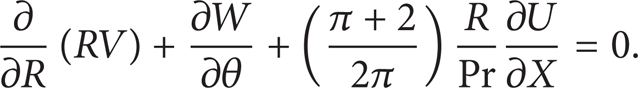
Continuity:

\frac{\partial}{\partial R} (R V) + \frac{\partial W}{\partial θ} + (\frac{π + 2}{2 π}) \frac{R}{Pr} \frac{\partial U}{\partial X} = 0 .

(3)

Axial Momentum:

[V \frac{\partial U}{\partial R} + \frac{W}{R} \frac{\partial U}{\partial θ} + (\frac{π + 2}{2 π}) \frac{U}{Pr} \frac{\partial U}{\partial X}] = - \frac{1}{Pr} \frac{d {\bar{P}}_{1}}{d X} (\frac{π + 2}{2 π}) + \nabla^{2} U + \frac{2 π}{(π + 2)} \frac{Gr}{Re} T \sin α .

(4)

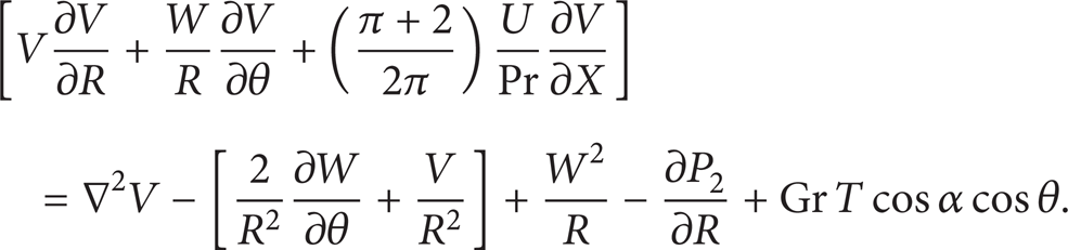
Radial Momentum:

[V \frac{\partial V}{\partial R} + \frac{W}{R} \frac{\partial V}{\partial θ} + (\frac{π + 2}{2 π}) \frac{U}{Pr} \frac{\partial V}{\partial X}] = \nabla^{2} V - [\frac{2}{R^{2}} \frac{\partial W}{\partial θ} + \frac{V}{R^{2}}] + \frac{W^{2}}{R} - \frac{\partial P_{2}}{\partial R} + Gr T \cos α \cos θ .

(5)

Angular Momentum:

[V \frac{\partial W}{\partial R} + \frac{W}{R} \frac{\partial W}{\partial θ} + (\frac{π + 2}{2 π}) \frac{U}{Pr} \frac{\partial W}{\partial X}] = \nabla^{2} W + [\frac{2}{R^{2}} \frac{\partial V}{\partial θ} - \frac{W}{R^{2}}] - \frac{W V}{R} - \frac{1}{R} \frac{\partial P_{2}}{\partial θ} - Gr T \cos α \sin θ .

(6)

Energy:

Pr [V \frac{\partial T}{\partial R} + \frac{W}{R} \frac{\partial T}{\partial θ} + (\frac{π + 2}{2 π}) \frac{U}{Pr} \frac{\partial T}{\partial X}] = \nabla^{2} T,

(7)

where

\nabla^{2} = \frac{1}{R} \frac{\partial}{\partial R} (R \frac{\partial}{\partial R}) + \frac{1}{R^{2}} \frac{\partial^{2}}{\partial θ^{2}} .

(8)

With dimensionless parameters of

{\begin{matrix} R = \frac{r}{r_{0}}, X = \frac{x}{r_{0} PrRe}, V = \frac{v r_{0}}{ν}, W = \frac{w r_{0}}{ν}, U = \frac{u}{u_{b}} \\ T = \frac{t - t_{e}}{\bar{q} / k}, {\bar{P}}_{1} = \frac{{\bar{p}}_{1}^{*}}{ρ u_{b}^{2}}, P_{2} = \frac{p_{2}^{*} r_{0}^{2}}{ρ ν^{2}} \\ Re = \frac{D_{h} u_{b}}{ν}, Pr = \frac{ρ ν C_{p}}{k}, Gr = \frac{g β \bar{q} r_{0}^{3}}{k ν^{2}}, D_{h} = (\frac{2 π}{π + 2}) r_{0} \end{matrix}}

(9)

the dimensionless initial conditions are:

{\begin{matrix} U = 1 & with in the fluid \\ U = 0 & at the walls \\ T = 0 & for all R and θ \\ {\bar{P}}_{1} = {\bar{P}}_{0} & with in the fluid \\ V = W = P_{2} = 0 & for all R and θ \end{matrix}} .

(10)

The dimensionless boundary conditions are

{\begin{Bmatrix} U = V = W = 0 & at the walls \\ T = T_{w} & at the walls \end{Bmatrix}} .

(11)

Starting from uniform flow at the inlet of the duct (defined by (10)) the solution for $U, V, W, {\bar{P}}_{1}$ , P₂, and T is to be determined as a function of X, R, and θ. The solution is to be progressed along X until X = 0.2 for all Gr. This distance is sufficient to insure that the fully developed region has been reached, which is consistent with the experimental observations of [19] in which the majority of the runs reached the fully developed region for X less than 0.1.

Some important engineering relations have been put in dimensionless form:

N u_{x} = \frac{h D_{h}}{k} = \frac{2 π}{{(π + 2)}^{2}_{}} \frac{1}{(T_{w} - T_{b})} .

(12)

The product fRe_x, where the friction factor f is defined by

f = \frac{{\bar{τ}}_{w}}{(1 / 2) ρ {u_{b}^{2}}_{}} .

(13)

The parameter ${\bar{τ}}_{w}$ was calculated by averaging the wall shear stress around the circumference of the duct. Thus, the average wall friction factor is as given by [4]:

f {Re}_{x} = \frac{4 π}{{(π + 2)}^{2}} \times [\int_{0}^{1} {(\frac{\partial U}{R \partial θ})}_{θ = 0} d R - \int_{0}^{1} {(\frac{\partial U}{R \partial θ})}_{θ = π} d R - \int_{0}^{π} {(\frac{\partial U}{\partial R})}_{R = 1} d θ] .

(14)

3. Solution Procedure

A uniform staggered grid on the cross plane and nonuniform divisions in the axial direction were utilized to discretize the governing equations. The analytical formulations were performed by using the finite control volume approach. The axial step size was taken as ΔX = 10⁻⁵ near the duct inlet. Then ΔX was increased by 5% for each consecutive step until ΔX reaches the value of 10⁻³ which was then kept constant, while the subdivisions for R and θ were kept the same along the duct. The solution of the governing equations ((3) through (7)) was progressed along X, by employing the SIMPLER algorithm of Patankar [21]. These equations were solved for each radial line using the tridiagonal matrix algorithm (TDMA), and the domain was covered by sweeping line by line in the angular direction. In each run, iterations were continued until the three velocity components and the temperature at all nodal points as well as the values of fRe_x and Nu_x satisfied the following convergence criteria:

| \frac{ϕ_{new} - ϕ_{old}}{ϕ_{new}} | < 1 0^{- 5} .

(15)

The decision about the mesh size was guided from the results of pure forced Nu_o and fRe_o in the developing and fully developed regions at Gr = 0. After extensive experimentation, the grid 30 × 50 was selected since it appears to be adequate for this study. Comparing the exact solution of Nu_o = 4.088 as in [22] and fRe_o = 15.767 as in [23]. With this grid, the present numerical results are within 0.12% and 0.1% for (Nu_o)_fd and (fRe_o)_fd, respectively.

For the given value of Gr (e.g., Gr = 10⁷) and Pr = 4, the fully developed Nu_fd and fRe_fd for mixed convection were compared with [3, 24] for horizontal and inclined semicircular ducts, respectively. Table 1 shows the comparison for both horizontal and inclined semicircular ducts at Gr = 10⁷.

Table 1:

Comparison of fully developed Nu and fRe with [3, 24] for Gr = 10⁷.

Inclination angle	α = 0°		α = 20°
Inclination angle	Nu_fd	fRe _fd	Nu_fd	fRe _fd

Present	17.973	24.695	18.922	24.108
[3]	17.983	24.708	—	—
[24]	—	—	18.625	23.990

Figure 2 shows a comparison between the present results and those of Lei and Trupp [25] and Hong and Bergles [26] of the axial variation of Nu_x for the case of forced convection (Gr = 0). The present results are in good agreement with the results of [25, 26]. The noticeable difference is limited to a very small region near the entrance where, X < 7 × 10⁻⁴. This is due to the fact that our model assumes simultaneously developing the temperature and velocity profiles, while [25, 26] assume fully developed velocity profile and developing temperature profile.

Figure 2:

Variation of Nu_x for forced convection (Gr = 0).

4. Results

The numerical investigations were carried out with Pr = 7, Re = 500, α = 0°, 20° and a wide range of Gr. These investigations include the development of velocity and temperature profiles and the development of overall quantities fRe_x and Nu_x with the axial coordinate.

4.1. Axial Velocity Development

Figure 3 shows the development of the axial velocity contours for the case of forced convection (Gr = 0). The flow is symmetric due to the absence of free convection, and the maximum velocity is moved toward the center of the duct cross section as the flow approaches the fully developed state. The development of axial velocity contours for the case of Gr = 10⁷ and α = 0° is shown in Figure 4. In the absence of buoyancy effects, the isovels are seen to be very much similar to those of pure forced convection. The velocity is constant in most of the flow domain with sharp changes very near the duct walls as shown in station (I). As the flow precedes further downstream in stations (II) and (III), the effects of buoyancy begin to appear. As it can be seen that, the maximum velocity shifts downward towards the lower part of the duct cross-section due to the secondary flow motion generated by the effect of free convection and significant velocity gradient developed in the middle part of the duct. In station (IV), the velocity profile has almost reached the fully developed state and the maximum velocity confined in the lower part of the duct. In station (V) the boundary layer is completely established and the fully developed state has been reached.

Figure 3:

Axial velocity contours at different axial stations for Gr = 0.

Figure 4:

Axial velocity contours at different axial stations for Gr = 10⁷ and α = 0°.

Figure 5 shows the development of isovels for the case of Gr = 10⁷ and α = 20°. The flow in station (I) is similar to the one of the horizontal case. As the flow proceeds to station (II), the buoyancy effects begin to appear by distorting the symmetry of the flow and moving the maximum velocity towards the lower part of the duct, and part of the flow with high momentum moves upward due to the axial component of the buoyancy force. In station (III), higher momentum fluid continues to move upwards. Stations (II) and (III) are characterized with high velocity gradient all over the duct walls. Thus the flow in these two stations produces higher friction factors than those of the horizontal case, as it will be shown later. As the flow reaches station (IV) the maximum velocity moves upward with greater velocity gradient in the upper part of the duct cross section. The flow then becomes fully developed as it reaches station (V) and the maximum velocity confined in the upper part of the duct.

Figure 5:

Axial velocity contours at different axial stations for Gr = 10⁷ and α = 20°.

4.2. Development of Temperature Profiles

Figure 6 shows the development of temperature contours for the case of the forced convection (Gr = 0). The flow is symmetric and the minimum temperature moves toward the center of the duct as the flow proceeds toward the fully developed state. Figure 7 shows the development of (T – T_w) contours for the case of Gr = 10⁷ and α = 0°. In station (I), the temperature contours are seen to be very much similar to those of pure forced convection. The temperature is constant in the most of the flow domain with sharp changes very near the duct walls. As the flow moves further downstream, station (II), the symmetry of the temperature distribution is distorted indicating a free convection effect. As the flow proceeds further downstream in stations (III) and (IV), the minimum (T – T_w) temperature shifts downward towards the lower part of the duct, and the area occupied by the cooler fluid is reduced indicating a higher heat transfer rate than that of station (II). When the fluid reached station (V) downstream which is far from the entrance, the flow is fully developed with a minimum (T – T_w) located in the lower corner of the duct.

Figure 6:

Temperature contours, (T – T_w) at different axial stations for Gr = 0.

Figure 7:

Temperature contours, (T – T_w) at different axial stations for Gr = 10⁷ and α = 0°.

Figure 8 shows the development of (T – T_w) temperature contours for Gr = 10⁷ and α = 20°. The development is similar to that of horizontal case except that the area occupied by the cooler fluid is reduced as compared with the horizontal case, particularly in the last two stations. This is because of the higher strength of the secondary flow for the upward inclination resulting in higher heat transfer rate, as it will be shown later.

Figure 8:

Temperature contours, (T – T_w) at different axial stations for Gr = 10⁷ and α = 20°.

4.3. Effect of Grashof Number

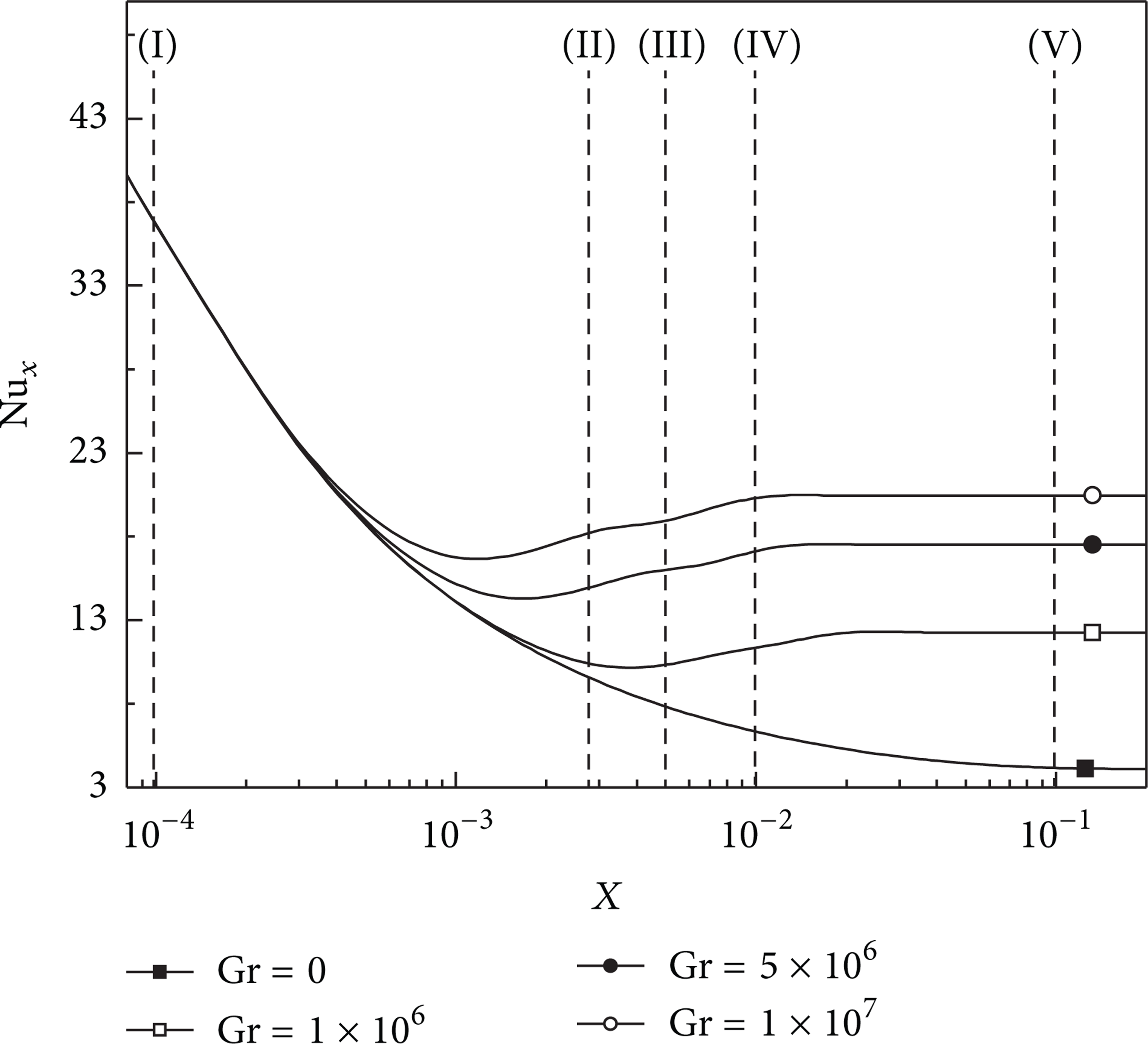
The effect of Gr on the Nu_x is presented in Figure 9 for α = 0°. At smaller values of X, Nu_x values are very close to the forced convection values due to the absence of free convection. As X increases, Nu_x decreases to a local minimum and then rises up to the fully developed value. This is due to the generation of strong currents of the secondary flow. Further, as Gr increases the minimum Nu_x value shifts upstream. This behavior is predicted experimentally by Maughan and Incropera [17] for horizontal and inclined parallel plates, Busedra and Soliman [19] for inclined semicircular ducts, and numerically by Mahaney et al. [10] for rectangular ducts. The increase in Gr enhances Nu_x in the developing and fully developed regions. The corresponding values of Nu_x at stations (III) and (V) for Gr = 1 × 10⁷ are 18.9631 and 20.4597, respectively, which are 243%, 491% higher than those of forced convection at the same axial stations. Figure 10 shows the effect of Gr on Nu_x for the case of α = 20°. The trend is quite the same as that of α = 0° with enhancement in Nu_x for both the developing and fully developed regions. At Gr = 10⁷, the corresponding values of Nu_x at stations (III) and (V) are 21.4944 and 21.5734, respectively, which are 275.5%, 518% higher than those of forced convection at the same axial stations.

Figure 9:

Effect of Gr on Nu_x for α = 0°.

Figure 10:

Effect of Gr on Nu_x for α = 20°.

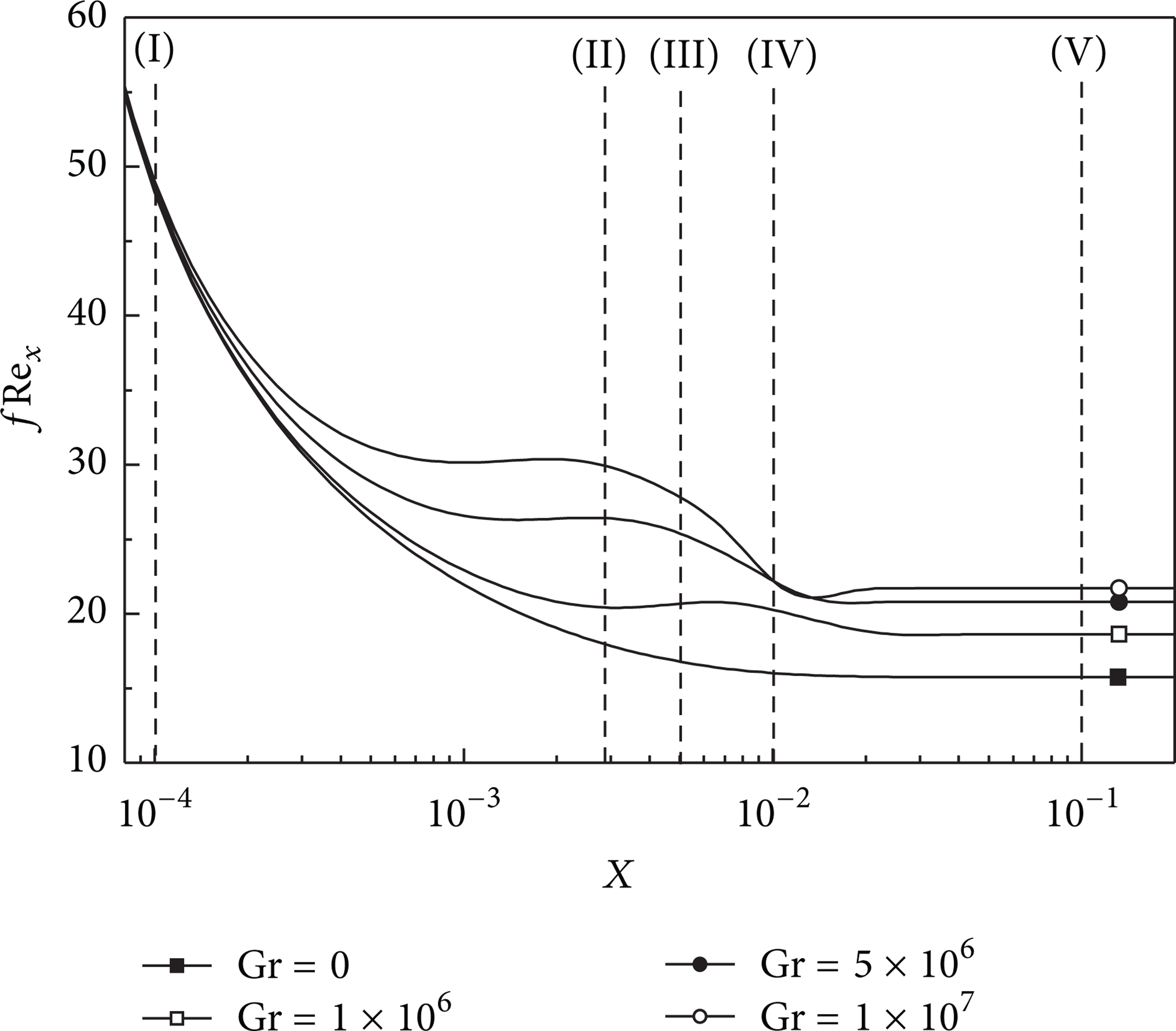
Figure 11 shows the effect of Gr on fRe_x for the case of α = 0°. Generally, fRe_x increases in the developing and fully developed regions with Gr, but the increase is much higher in the developing region. Again due to the absence of free convection, the values of fRe_x near the entrance are close to the forced convection values. As X increases downstream, the values of fRe_x start deviating from the forced convection values due to the active secondary flow currents. As X increases further, the values of fRe_x decreases until it reaches a constant value (fully developed). The values of fRe_x are higher in the developing region than those in the fully developed region. Figure 12 shows the effect of Gr on fRe_x for α = 20°. The trend is similar to that of the horizontal duct. Beyond station (IV), however, fRe_x drops as Gr increases up to a critical value, and then it increases as Gr increases until it reaches the constant fully developed value.

Figure 11:

Effect of Gr on fRe_x for α = 0°.

Figure 12:

Effect of Gr on fRe_x for α = 20°.

4.4. Comparison between Horizontal and Inclined Ducts

Figure 13 shows the effect of inclination angle on the development of Nu_x. The values of Nu_x for α = 20° are higher than that of α = 0° in most part of the duct length. This can be contributed to the fact that the axial component of the buoyancy in the flow direction accelerates the fluid which results in higher heat transfer rate. In addition to that, the inclination effect is more pronounced in the developing region than in the fully developed region.

Figure 13:

Effect of inclination angle on Nu_x for Gr = 10⁷.

The effect of inclination on fRe_x is shown Figure 14. The values of fRe_x are much higher for the inclined duct than those of horizontal duct in the developing region because of the axial velocity profiles characterized by high velocity gradient near the walls for almost all the duct cross section. However, as the flow proceeds further fRe_x decreases until it approaches the curve of the horizontal duct in the fully developed region. In this region, the values of fRe_x for horizontal and inclined ducts are almost equal. This is due to the fact that the velocity gradient for the two cases is distributed around the wall in a similar fashion, with a difference in the location of maximum velocity being at the upper half of the duct section for the inclined and at the lower half of the duct for the horizontal case, as shown previously. The axial temperature distribution for the case of horizontal and inclined duct is presented in Figure 15. The wall temperature to fluid bulk temperature differences are always lower for α = 20° than that of α = 0° for most of the duct length. This indicates that Nu_x is always higher for α = 20° than that of α = 0°.

Figure 14:

Effect of inclination angle on fRe_x for Gr = 10⁷.

Figure 15:

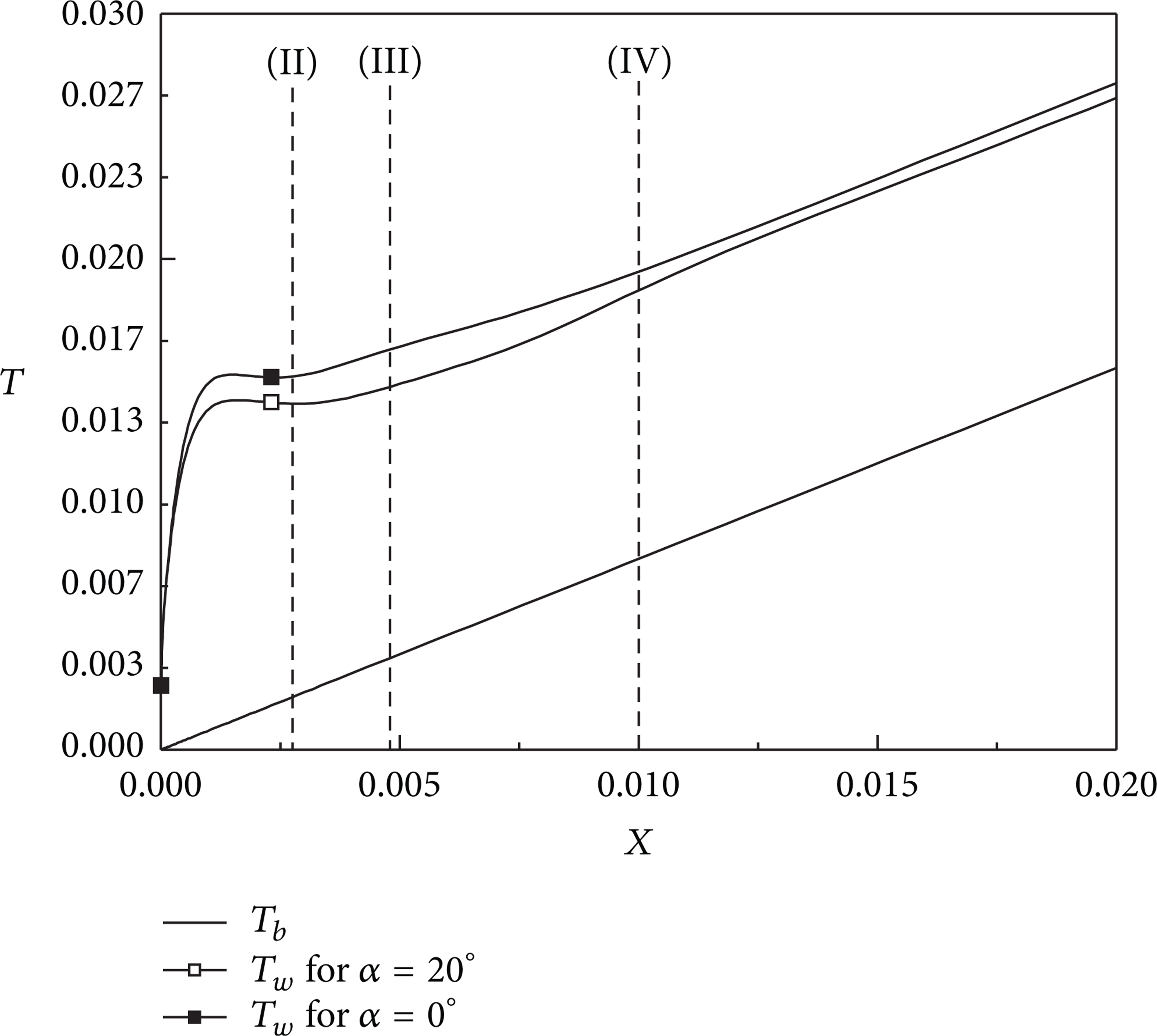
Variation of T_w and T_b along the duct for Gr = 10⁷.

4.5. Comparison of Present Prediction with Experimental Results

The present work is compared with the experimental results of [19] for thermally developing and fully developed regions. All theoretical predictions are generated for the average Pr and Gr for the respective experimental data set with Re = 500. The general trend of the present results for the horizontal and inclined cases is consistent with the experimental results of [19], as shown in Figures 16 and 17. Figure 16 shows that the present results, for the case of α = 0°, approach well the experimental results in the early part of the duct, where the effect of free convection is weak while in the fully developed region the theoretical results slightly deviate from the experimental data. However, at high Grashof number, (e.g., Gr = 1.24 × 10⁷) the deviation is more pronounced in the developing region, as shown in Figure 16. This may be attributed to the assumption of simultaneously developing and uniform wall temperature circumferentially. This may not be achieved accurately as in the experiments especially with high Gr due to some heat loss and circumferential variation in wall temperature. The maximum deviation between the theoretical and experimental results is 15% at X = 0.0034 for Gr = 1.24 × 10⁷ with Pr = 5.74. The inclined case is represented in Figure 17. The trend is similar to that of the horizontal case. It can be seen that some of the experimental data exceeds the theoretical curves in the fully developed region. The maximum deviation between the theoretical and the experimental results is about 18% at X = 0.0034 for Gr = 1.22 × 10⁷ with Pr = 5.76.

Figure 16:

Comparison of present results of Nu_x with the experimental results for α = 0°.

Figure 17:

Comparison of present results of Nu_x with the experimental results for α = 20°.

5. Conclusions

An investigation of laminar mixed convection has been utilized for solving the entrance region of simultaneously developing hydrodynamically and thermally in horizontal and inclined semicircular ducts for H1 thermal boundary condition. The test matrix for which the results were obtained included two inclination angles (α = 0° and 20°), Re = 500, Pr = 7.0, and wide range of Gr. From these results, the following conclusions can be made.

Nu_x and fRe_x increase in the developing and fully developed regions with Gr.

Nu_x decreases in the developing region up to a critical value. Beyond that, it starts increasing in both developing and fully developed regions. The general trend of the axial variation of Nu_x is similar to those noted in the previous work for horizontal and inclined ducts.

The axial variation of fRe_x is different from that of Nu_x. fRe_x is found to be decreasing along the duct length in the developing and fully developed regions. In addition, fRe_x values in the developing region are higher for α = 20° than that of α = 0°.

The inclination angle has a stronger influence in the developing of the axial velocity profiles rather than the temperature profiles.

The inclined duct produces higher Nu_x in the developing and fully developed regions and higher fRe_x values in the developing region, while in the fully developed region the fRe_x values are the same as in the horizontal case.

The present results of Nu_x are consistent with the experimental results of [19] for both horizontal and inclined semicircular ducts. For both cases of α = 0° and 20°, the present work approaches the experimental results well in the early part of the duct, while in the fully developed region the theoretical results deviate from the experimental data, particularly at higher Gr.

Footnotes

Nomenclature

References

Nandakumar

Masliyah

J. H.

, and Law

H. S.

, “Bifurcation in steady laminar mixed convection flow in horizontal ducts,” Journal of Fluid Mechanics, vol. 152, pp. 145–161, 1985.

Lei

Q. M.

and Trupp

A. C.

, “Predictions of laminar mixed convection in a horizontal semicircular duct,” in Proceedings of the 6th International Symposium on Heat and Mass Transfer, pp. 10–12, Miami, Fla, USA, 1990.

Chinproncharoenpong

Trupp

A. C.

, and Soliman

H. M.

, “Effect of gravitational force orientation on laminar mixed convection for a horizontal semicircular duct,” in Proceedings of the 3rd World Conference on Experimental Heat Transfer, Fluid Mechanics and Thermodynamics, pp. 131–137, Elsevier, 1993.

Busedra

A. A.

and Soliman

H. M.

, “Analysis of laminar mixed convection in inclined semicircular ducts under buoyancy-assisted and -opposed conditions,” Numerical Heat Transfer A, vol. 36, no. 5, pp. 527–544, 1999.

Cheng

C. H.

Lin

C. Y.

, and Aung

, “Predictions of developing flow with buoyancy-assisted flow separation in a vertical rectangular duct: parabolic model versus elliptic model,” Numerical Heat Transfer A, vol. 37, no. 6, pp. 567–586, 2000.

Cheng

C. H.

Aung

, and Weng

C. J.

, “Buoyancy-assisted flow reversal and convective heat transfer in entrance region of a vertical rectangular duct,” International Journal of Heat and Fluid Flow, vol. 21, no. 4, pp. 403–411, 2000.

Cheng

C. H.

Huang

S. Y.

, and Aung

, “Numerical predictions of mixed convection and flow separation in a vertical duct with arbitrary cross section,” Numerical Heat Transfer A, vol. 41, no. 5, pp. 491–514, 2002.

Nesreddine

Galanis

, and Nguyen

C. T.

, “Effects of axial diffusion on laminar heat transfer with low péclet numbers in the entrance region of thin vertical tubes,” Numerical Heat Transfer A, vol. 33, no. 3, pp. 247–266, 1998.

Zeldin

and Schmidt

F. W.

, “Developing flow with combined forced-free convection in an isothermal vertical tube,” Journal of Heat Transfer, vol. 94, no. 2, pp. 211–223, 1972.

10.

Mahaney

H. V.

Incropera

F. P.

, and Ramadhyani

, “Development of laminar mixed convection flow in a horizontal rectangular duct with uniform bottom heating,” Numerical Heat Transfer A, vol. 12, no. 2, pp. 137–155, 1987.

11.

Islam

Gaitonde

U. N.

, and Sharma

G. K.

, “Mixed convection heat transfer in the entrance region of horizontal annuli,” International Journal of Heat and Mass Transfer, vol. 44, no. 11, pp. 2107–2120, 2001.

12.

Nguyen

C. T.

and Galanis

, “Combined forced and free convection for the developing laminar flow in horizontal tubes under uniform heat flux,” in Proceedings of the Numerical Methods in Thermal Problems Conference, vol. 5, part A, pp. 414–425, Montreal, Canada, 1986.

13.

Naito

and Nagano

, “Combined forced and free upward-flow convection in the entrance region between inclined parallel plates,” Journal of Heat Transfer, vol. 111, no. 3, pp. 675–682, 1989.

14.

Morcos

S. M.

and Abou-Ellail

M. M. M.

, “Buoyancy effects in the entrance region of an inclined multirectangular-channel solar collector,” Journal of Solar Energy Engineering, vol. 105, no. 2, pp. 157–163, 1983.

15.

Barozzi

G. S.

Zanchini

, and Mariotti

, “Experimental investigation of combined forced and free convection in horizontal and inclined tubes,” Meccanica, vol. 20, no. 1, pp. 18–27, 1985.

16.

Morcos

S. M.

Hilal

M. M.

Kamel

M. M.

, and Soliman

M. S.

, “Experimental investigation of mixed laminar convection in the entrance region of inclined rectangular channels,” Journal of Heat Transfer, vol. 108, pp. 574–579, 1986.

17.

Maughan

J. R.

and Incropera

F. P.

, “Experiments on mixed convection heat transfer for airflow in a horizontal and inclined channel,” International Journal of Heat and Mass Transfer, vol. 30, no. 7, pp. 1307–1318, 1987.

18.

Lei

Q. M.

and Trupp

A. C.

, “Experimental study of laminar mixed convection in the entrance region of a horizontal semicircular duct,” International Journal of Heat and Mass Transfer, vol. 34, no. 9, pp. 2361–2372, 1991.

19.

Busedra

A. A.

and Soliman

H. M.

, “Experimental investigation of laminar mixed convection in an inclined semicircular duct under buoyancy assisted and opposed conditions,” International Journal of Heat and Mass Transfer, vol. 43, no. 7, pp. 1103–1111, 2000.

20.

Anderson

D. A.

Tannehill

J. C.

, and Pletcher

R. H.

, Computational Fluid Mechanics and Heat Transfer, McGraw-Hill, New York, NY, USA, 1984.

21.

Patankar

S. V.

, Numerical Heat Transfer and Fluid Flow, McGraw Hill, New York, NY, USA, 1980.

22.

Lei

Q. M.

and Trupp

A. C.

, “Further analysis of laminar flow heat transfer in circular sector ducts,” Journal of Heat Transfer, vol. 111, pp. 1088–1090, 1989.

23.

Lei

Q. M.

and Trupp

A. C.

, “Maximum velocity location and pressure drop of fully developed laminar flow in circular sector ducts,” Journal of Heat Transfer, vol. 111, pp. 1085–1087, 1989.

24.

Abeedy

E. A. El.

, Effect of orientation on laminar mixed convection for inclined semicircular ducts [M.S. thesis], University of Garyounis, Benghazi, Libya, 2004.

25.

Lei

Q. M.

and Trupp

A. C.

, “Forced convection of thermally developing laminar flow in circular sector ducts,” International Journal of Heat and Mass Transfer, vol. 33, no. 8, pp. 1675–1683, 1990.

26.

Hong

S. W.

and Bergles

A. E.

, “Augmentation of laminar flow heat transfer in tubes by means of twisted-tape inserts,” Tech. Rep. HTL-S, ISU-ERI-Ames-75011, Engineering Research Institute, Iowa State University, Ames, Iowa, USA, 1974.

Laminar Mixed Convection in the Entrance Region of Horizontal and Inclined Semicircular Ducts

Abstract

1. Introduction

2. Mathematical Model

3. Solution Procedure

4. Results

4.1. Axial Velocity Development

4.2. Development of Temperature Profiles

4.3. Effect of Grashof Number

4.4. Comparison between Horizontal and Inclined Ducts

4.5. Comparison of Present Prediction with Experimental Results

5. Conclusions

Footnotes

Nomenclature

References