Sage Journals: Discover world-class research

Abstract

The NCS (networked control system) is different from the conventional control systems which is the integration of the automation and control over communication network. When an NCS operates over the communication network, one of the major challenges is the network-induced delay in data transfer among the controllers, actuators, and sensors. This delay degrades system performance and causes system unstablility. This paper proposes a GPC (generalized predictive control) with the Kalman state estimator to compensate for the network-induced delay and packet loss. The GPC is implemented in WiNCS (Wireless NCS) based on IEEE 802.11 standard. An analytical NCS model and NS2 (network simulator version 2) are developed to simulate and evaluate the performance under the effect of various delays and packet loss rates. The result shows that the proposed GPC is adaptive and robust to the uncertainties in a time-delay system. The WiNCS is evaluated with latency and throughput measurements in various environments. The experiment setup conforming to the IEEE 802.11 standard achieves an average latency of 1.3 ms and a data throughput of 3.000 kB/s up to a distance of 70 m. The results demonstrate the feasibility of real-time closed-loop control with the proposed concept.

1. Introduction

In recent years, there has been an increasing interest in implementing networked transmission protocols (e.g., wire/wireless local area networks) in automation and control system. Cost effectiveness and flexibility are achieved using communication protocol in the feedback control.

The NCS closes the feedback control loops through a real-time network. The control signals to the actuators and the feedback signals from sensors are in the form of information packages [1, 2]. Interconnecting the sensors, actuators, and controllers via networks can eliminate wiring, reduce installation costs, and enable remote monitoring and tuning. Additional components and modules can be added without additional circuitry to the existing layout. The controllers effectively share the data via the information technology allowing easy data fusion and integration to the controller for an intelligent decision or optimal operation in a large and complex process [3, 4]. The potential applications of NCS include industrial automation, military, hazardous environment exploration, or robots application.

Three methods on scheduling packets were proposed to improve NCS performance and stability as static scheduler, try-once-discard (TOD) scheduler with continuous priority level, and TOD with discrete priority level [5, 6].

A networked DC motor control system was proposed using controller gain adaptation to compensate the changes in QoS (quality-of-service) requirements over time-varying network [7].

Stabilization of NCS was investigated in the discrete-time domain with random delays [8]. Two Markov chains were applied to model the delay on controller-to-actuator delay and sensor-to-controller.

Model-based NCS was proposed using an explicit model of the plant to produce an estimate of the plant state during transmission delay. The stability was evaluated for the controller/actuator which was updated with sensor information at nonconstant time intervals [9].

An NCS model including network-induced delay and packet loss in transmission network was proposed. The feedback gain of a memory-less controller and the maximum allowable value of the network-induced delay were derived by solving a set of linear matrix inequalities [10]. Two predictors estimating the plant outputs in open-loop and closed-loop were proposed [11].

An error predictive model was built using a back propagation neural network to reduce the error on estimation of output. Three control methods were compared as PID, GPC, and GPC with error correction. GPC with error correction was validated to have the best performance [12].

A novel GPC strategy was proposed controlling NCS with respect to the NSC structure characteristics. The timestamp mechanism of data communication network was applied. Accurate measurement to the system output and timely modification to the predictive value were required under the random network-induced delay [13].

A client-server control architecture was implemented on the dual-axis hydraulic position system of an industrial fish-processing machine. The GPC algorithm was adopted to compensate for data-transmission delays. It incorporates a minimum-effort estimator to estimate missing or delayed sensor data and a variable-horizon adaptive GPC controller to predict the required future control efforts to drive the plant to track a desired reference trajectory [14].

Time-varying delays for the transmission of sensor and control signal over the wireless network were evaluated using a randomized multihop routing protocol. The proposed predictive control scheme with a delay estimator was based on a Kalman filter [15].

This paper presents a model of the NCS with network-induced delay and packets loss for a general SISO NCS model. The stochastic time delays reduce the system performance (e.g., stability, controllability, and observability). This paper applies GPC to predict the network-induced delay and simulate it through the wireless network environment setup by NS2 in Linux. The PiccSIM is used as the platform in the client/server architecture for the WiNCS. The MPC concept was adopted and the GPC control algorithm with the Kalman state estimator is implemented in WiNCS to reduce the effect on network-induced delay and packets loss.

The contributions in the paper are summarized as follows. (i)

The main factors affecting the performance of NCS in communication networks have been identified.

(ii)

The NCS with network-induced delay and packet loss is modeled.

(iii)

The GPC algorithm is implemented in WiNCS to cope with the time-varying delay issue.

(iv)

The simulated platform is constructed which connects NS2 and Matlab∖Simulink for implementation of GPC in WiNCS.

2. Method

The GPC is proposed to compensate the network-induced delay in WiNCS. The algorithm, closed-loop structure, and CARIMA model structure are developed. The GPC in state space with state estimator is derived for WiNCS simulation. The state space is adopted to reduce the algebraic complexity in the GPC control law.

2.1. Formulation of GPC

The SISO (single-input single-output) system is given which considers the operation around a specific set point after linearization. A predictive model known as CARIMA (controlled autoregressive integrated moving average) for GPC is

\begin{matrix} A (z^{- 1}) y (k) = B (z^{- 1}) u (k - 1) + \frac{C (z^{- 1})}{Δ} e (k), \end{matrix}

(1)

with

\begin{matrix} Δ = 1 - z^{- 1}, \end{matrix}

(2)

where

y (k)

is output signal,

u (k)

is input signal,

e (k)

is zero mean white noise, and A, B, and C are

\begin{matrix} A (z^{- 1}) = 1 + a_{1} z^{- 1} + a_{2} z^{- 2} + \dots + a_{n a} z^{- n a} \\ B (z^{- 1}) = b_{0} + b_{1} z^{- 1} + b_{2} z^{- 2} + \dots + b_{n b} z^{- n b} \\ C (z^{- 1}) = 1 + c_{1} z^{- 1} + c_{2} z^{- 2} + \dots + c_{n c} z^{- n c}, \end{matrix}

(3)

where

C (z^{- 1})

is selected to be 1 for the simplicity. The cost function including the influence of

u (k)

on future system is to enhance the system robustness. GPC algorithm applies a control sequence to minimize a multistage cost function as

\begin{array}{l} J = \sum_{j = n_{1}}^{n_{2}} δ (j) {[\hat{y} (k + j) - w (k + j)]}^{2} \\ + \sum_{j = 1}^{H_{c}} λ (j) {[Δ u (k + j - 1)]}^{2}, \end{array}

(4)

where

\hat{y} (k + j)

is optimum j-step ahead prediction of system output,

n_{1}

and

n_{2}

are the minimum and maximum of the prediction horizons

H_{p}

and the order of

n_{2}

must be larger than

B (z^{- 1})

H_{c}

is control horizon

{(H_{c} \leq H}_{p})

δ (j)

and

λ (j)

are weighting sequences,

δ (j)

is selected to be 1, and

λ (j)

is a constant.

w (k + j)

is the future reference trajectory as

\begin{matrix} w (k + j) = α^{j} y (k + j) + (1 - α^{j}) y_{r} (j = 1,2, 3 \dots, n), \end{matrix}

(5)

where

y (k)

and

y_{r}

are the set point and the future output of the system, respectively. α is a parameter between 0 and 1 that affects the response of the system (closer to 1, smoother response curve).

The optimal prediction of the output $y (k + j)$ is driven close to $w (k + j)$ to optimize the cost function. Diophantine equation for predicting the precede j-step output is given by

\begin{matrix} 1 = E_{j} (z^{- 1}) \tilde{A} (z^{- 1}) + z^{- j} F_{j} (z^{- 1}), \end{matrix}

(6)

with

\begin{array}{l} \tilde{A} (z^{- 1}) = Δ A (z^{- 1}) = 1 + {\tilde{a}}_{1} z^{- 1} + {{\tilde{a}}_{2} z}^{- 2} \\ + \dots + {\tilde{a}}_{n a + 1} z^{- (n a + 1)}, \end{array}

(7)

where

\begin{matrix} E_{j} (z^{- 1}) = e_{j, 0} + e_{j, 1} z^{- 1} + e_{j, 2} z^{- 2} + \dots + e_{j, j - 1} z^{- (j - 1)} \\ F_{j} (z^{- 1}) = f_{j, 0} + f_{j, 1} z^{- 1} + f_{j, 2} z^{- 2} + \dots + f_{j, n a} z^{- n a} . \end{matrix}

(8)

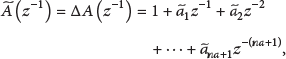
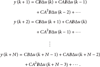
Equation (1) is multiplied by $Δ E_{j} (z^{- 1}) z^{j}$ to obtain the predictive equation of j-step after time k as

\begin{array}{l} \tilde{A} (z^{- 1}) E_{j} (z^{- 1}) y (k + j) = E_{j} (z^{- 1}) B (z^{- 1}) Δ u (k + j - 1) \\ + E_{j} (z^{- 1}) e (k + j) . \end{array}

(9)

Equation (9) is rewritten in consideration of (6) as

\begin{array}{l} y (k + j) = F_{j} (z^{- 1}) y (k) + E_{j} (z^{- 1}) B (z^{- 1}) \\ \times Δ u (k + j - 1) + E_{j} (z^{- 1}) e (k + j) . \end{array}

(10)

Noise term in the future on the system is neglected in (10). Letting $G_{j} (z^{- 1}) = E_{j} (z^{- 1}) B (z^{- 1})$ , the best prediction of future output is

\begin{matrix} \hat{y} (k + j) = G_{j} (z^{- 1}) Δ u (k + j - 1) + F_{j} (z^{- 1}) y (k) . \end{matrix}

(11)

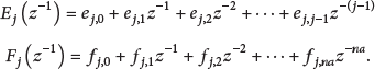
The set of the control signals $u (k), u (k + 1), \dots, u (k + N)$ is obtained to optimize (4). The values $n_{1}$ , $n_{2}$ , and $H_{c}$ are defined by $n_{1} = 1$ and $n_{2} = N$ and the predictive horizon $H_{p} = N$ and the control horizon $H_{c} = N$ . N ahead optimal prediction is considered as

\begin{matrix} \hat{y} (k + 1) = G_{1} Δ u (k) + F_{1} (z^{- 1}) y (k) \\ \hat{y} (k + 2) = G_{2} Δ u (k + 1) + F_{2} (z^{- 1}) y (k) \\ \hat{y} (k + 3) = G_{3} Δ u (k + 2) + F_{3} (z^{- 1}) y (k) \\ ⋮ \\ \hat{y} (k + N) = G_{N} Δ u (k + N - 1) + F_{N} (z^{- 1}) y (k) . \end{matrix}

(12)

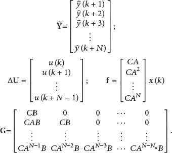
The above equations are marshaled as

\begin{matrix} \hat{Y} = G Δ U + F (z^{- 1}) y (k) + H (z^{- 1}) Δ u (k - 1), \end{matrix}

(13)

where

\begin{array}{l} \hat{Y} = [\begin{bmatrix} \hat{y} (k + 1) \\ \hat{y} (k + 2) \\ \hat{y} (k + 3) \\ ⋮ \\ \hat{y} (k + N) \end{bmatrix}]; G = [\begin{bmatrix} g_{0} & 0 & \dots & 0 \\ g_{1} & g_{0} & \dots & 0 \\ ⋮ & ⋮ & ⋮ & ⋮ \\ g_{N - 1} & g_{N - 2} & \dots & g_{0} \end{bmatrix}]; \\ Δ U = [\begin{bmatrix} u (k) \\ u (k + 1) \\ ⋮ \\ u (k + N - 1) \end{bmatrix}]; F (z^{- 1}) = [\begin{bmatrix} F_{1} (z^{- 1}) \\ F_{2} (z^{- 1}) \\ ⋮ \\ F_{N} (z^{- 1}) \end{bmatrix}] \\ H (z^{- 1}) \\ = [\begin{bmatrix} (G_{1} (z^{- 1}) - g_{0}) z \\ (G_{2} (z^{- 1}) - g_{0} - g_{1} z^{- 1}) z^{2} \\ ⋮ \\ (G_{N} (z^{- 1}) - g_{0} - g_{1} z^{- 1} - \dots g_{N - 1} z^{- (N - 1)}) z^{N} \end{bmatrix}] . \end{array}

(14)

In (13), it includes known and unknown sequences at time k. The known sequence which is the last two terms is grouped into f as

\begin{matrix} \hat{Y} = G Δ U + f, \end{matrix}

(15)

where

\begin{matrix} f = F (z^{- 1}) y (k) + H (z^{- 1}) Δ u (k - 1) . \end{matrix}

(16)

Equation (4) is written in consideration (15) as

\begin{matrix} J = {(G Δ U + f - W)}^{T} (G Δ U + f - W) + λ {Δ U}^{T} Δ U, \end{matrix}

(17)

where

\begin{matrix} W = [\begin{bmatrix} w (k + 1) \\ w (k + 2) \\ ⋮ \\ w (k + N) \end{bmatrix}] . \end{matrix}

(18)

The minimum of J, assuming there are no constraints on the control signal, is found by taking gradient of J . Let $\partial J / \partial Δ U = 0$ which leads to

\begin{matrix} Δ U = {(G^{T} G + λ I)}^{- 1} G^{T} (W - f) . \end{matrix}

(19)

In (19), the actually control signal that is sent to the system is the first element of $Δ U$ as

\begin{matrix} u (k) = u (k - 1) + K (W - f), \end{matrix}

(20)

where

K = [\begin{bmatrix} k_{1} & k_{2} & \dots & k_{N} \end{bmatrix}]

is the first row of the matrix

{(G^{T} G + λ I)}^{- 1} G^{T}

The optimization in GPC is different from the general optimal algorithm; the optimized target is moving by time (i.e., local optimization in every sampling time). The first element of $Δ U$ is applied and the optimal procedure is repeated at the next sampling time [16, 17].

2.2. GPC Control Strategy

The following equations are rewritten to illustrate the GPC control block diagram. (a)

The reference trajectory in (5) is

\begin{matrix} W = Q y (k) + P y_{r}, \end{matrix}

(21)

where

Q = {[\begin{bmatrix} α & α^{2} & \dots & α^{n} \end{bmatrix}]}^{T}

and

P = {[\begin{bmatrix} 1 - α & {1 - α}^{2} & \dots & {1 - α}^{n} \end{bmatrix}]}^{T}

(b)

The predictive model (CARIMA) in (1) is

\begin{matrix} Δ A (z^{- 1}) y (k) = z^{- 1} B (z^{- 1}) Δ u (k) + C (z^{- 1}) e (k) . \end{matrix}

(22)

From (7) and (22), the CARIMA model is driven as

\begin{matrix} y (k) = \frac{z^{- 1} B}{A} u (k) + \frac{C}{A \cdot Δ} e (k), \end{matrix}

(23)

where the polynomial C is selected to be 1.

(c)

The predictive output in (16) is

\begin{matrix} f = F (z^{- 1}) y (k) + \bar{H} (z^{- 1}) Δ u (k), \end{matrix}

(24)

where

\begin{array}{l} \bar{H} (z^{- 1}) \\ = [\begin{bmatrix} (G_{1} (z^{- 1}) - g_{0}) \\ (G_{2} (z^{- 1}) - g_{0} - g_{1} z^{- 1}) z \\ ⋮ \\ (G_{N} (z^{- 1}) - g_{0} - g_{1} z^{- 1} - \dots g_{N - 1} z^{- (N - 1)}) z^{N - 1} \end{bmatrix}] . \end{array}

(25)

(d)

The control-increment vector is

\begin{matrix} Δ u (k) = K (W - f) . \end{matrix}

(26)

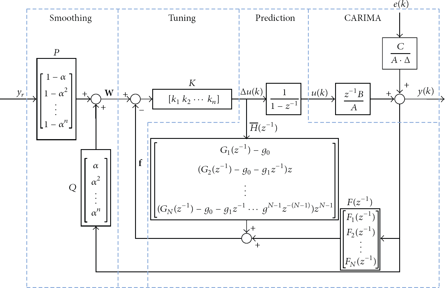
Figure 1 shows that the GPC control-loop structure consists of smoothing, tuning, and prediction processes. The thick line indicates the vector signal and the thin line indicates the scalar signal. At each moment, the desired output vector W is obtained after smoothing the set point $y_{r}$ . Compared with the predictive output and desired output, the declination vector is obtained. The control signal $Δ u$ at this moment is the product of declination vector and vector K. The control signal $Δ u$ also generates the new predictive output f with the vector $\bar{H}$ and the system output.

Figure 1

GPC control-loop structure.

2.3. GPC in State-Space Formulation

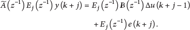
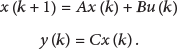
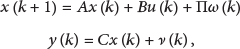
Consider a state-space description [18, 19] of the system plant which was given as follows. The dimension of the state vector is $n = \max (n_{a} + 1, n_{b} + 1, n_{c}) :$

\begin{matrix} x (k + 1) = A x (k) + B u (k) + Π ω (k) \\ y (k) = C x (k) + ν (k), \end{matrix}

(27)

where

\begin{matrix} A = [\begin{bmatrix} {- \tilde{a}}_{1} & 1 & 0 & \dots & 0 \\ {- \tilde{a}}_{2} & 0 & 1 & \dots & 0 \\ ⋮ & ⋮ & ⋮ & ⋮ & ⋮ \\ {- \tilde{a}}_{n} & 0 & 0 & \dots & 0 \\ ⋮ & ⋮ & ⋮ & ⋮ & ⋮ \\ {- \tilde{a}}_{n a + 1} & 0 & 0 & \dots & 0 \end{bmatrix}]; B = [\begin{bmatrix} 0 \\ 0 \\ ⋮ \\ b_{0} \\ ⋮ \\ b_{n b - 1} \end{bmatrix}]; \\ Π = [\begin{bmatrix} c_{1} {- \tilde{a}}_{1} \\ c_{2} {- \tilde{a}}_{2} \\ ⋮ \\ c_{n} {- \tilde{a}}_{n} \\ ⋮ \\ c_{n c} {- \tilde{a}}_{n c} \end{bmatrix}], C = [\begin{bmatrix} 1 & 0 & \dots & 0 & \dots & 0 & \dots \end{bmatrix}], \end{matrix}

(28)

where

{\tilde{a}}_{i}

are the coefficient of polynomial

\tilde{A}

. The random variables ω and ν represent disturbance input and measurement (sensor) noise, and they are assumed to be white Gaussian zero mean with normal probability distributions.

The noise and disturbance in (22) are neglected; the predictive model is rewritten as

\begin{matrix} x (k + 1) = A x (k) + B u (k) \\ y (k) = C x (k) . \end{matrix}

(29)

From (27), the z-domain transfer function $R (z)$ is derived as

\begin{array}{l} R (z) = C {(z I - A)}^{- 1} B \\ = \frac{C {(I - (A / z))}^{- 1} B}{z} = \frac{C}{z} (I + \frac{A}{z} + \frac{A^{2}}{z^{2}} + \frac{A^{3}}{z^{3}} + \dots) B \\ = \frac{C B}{z} + \frac{C A B}{z^{2}} + \frac{{C A}^{2} B}{z^{3}} + \frac{{C A}^{3} B}{z^{4}} + \dots . \end{array}

(30)

From (30), the current output is obtained as

\begin{array}{l} y (k) = C B Δ u (k - 1) + C A B Δ u (k - 2) \\ + {C A}^{2} B Δ u (k - 3) + \dots . \end{array}

(31)

Since the predictive horizon $H_{p} = N$ , the future output is obtained as

\begin{array}{l} y (k + 1) = C B Δ u (k) + C A B Δ u (k - 1) \\ + {C A}^{2} B Δ u (k - 2) + \dots \\ y (k + 2) = C B Δ u (k + 1) + C A B Δ u (k) \\ + {C A}^{2} B Δ u (k - 1) + \dots \\ ⋮ \\ y (k + N) = C B Δ u (k + N - 1) + C A B Δ u (k + N - 2) \\ + {C A}^{2} B Δ u (k + N - 3) + \dots . \end{array}

(32)

From the previous equations, the prediction state of the system is also obtained as

\begin{array}{l} x (k + 1) = A x (k) + B Δ u (k) \\ x (k + 2) = A x (k + 1) + B Δ u (k + 1) \\ = A^{2} x (k) + A B Δ u (k) + B Δ u (k + 1) \\ x (k + 3) = A^{3} x (k) + A^{2} B Δ u (k) \\ + A B Δ u (k + 1) + B Δ u (k + 2) \\ ⋮ \\ x (k + j) = A^{j} x (k) + \sum_{i = 1}^{j - 1} A^{j - i - 1} B Δ u (k + i) . \end{array}

(33)

A general term of $y (k + j)$ with $(j = 1,2, 3, \dots, N)$ is obtained as

\begin{array}{l} y (k + j) = \sum_{i = 1}^{\infty} {C A}^{i - 1} B Δ u (k + j - i) \\ = \sum_{i = 1}^{j} {C A}^{i - 1} B Δ u (k + j - i) \\ + \sum_{i = j + 1}^{\infty} {C A}^{i - 1} B Δ u (k + j - i) \\ = \sum_{i = 1}^{j} {C A}^{i - 1} B Δ u (k + j - i) \\ + \sum_{m = 0}^{\infty} {C A}^{m + j} B Δ u (k - m - 1) \\ = \sum_{i = 1}^{j} {C A}^{i - 1} B Δ u (k + j - i) \\ + \sum_{m = 0}^{\infty} {C A}^{m + j} [x (k - m) - A x (k - m - 1)] \\ = \sum_{i = 1}^{j} {C A}^{i - 1} B Δ u (k + j - i) \\ + \sum_{m = 0}^{\infty} {C A}^{j} [A^{m} x (k - m) - A^{m + 1} x (k - m - 1)] \\ = \sum_{i = 1}^{j} {C A}^{i - 1} B Δ u (k + j - i) + {C A}^{j} x (k) . \end{array}

(34)

Therefore, the predictive output is denoted as

\begin{matrix} \hat{Y} = G Δ U + f, \end{matrix}

(35)

where

\begin{matrix} \hat{Y} = [\begin{bmatrix} \hat{y} (k + 1) \\ \hat{y} (k + 2) \\ \hat{y} (k + 3) \\ ⋮ \\ \hat{y} (k + N) \end{bmatrix}]; \\ Δ U = [\begin{bmatrix} u (k) \\ u (k + 1) \\ ⋮ \\ u (k + N - 1) \end{bmatrix}]; f = [\begin{bmatrix} C A \\ {C A}^{2} \\ ⋮ \\ {C A}^{N} \end{bmatrix}] x (k) \\ G = [\begin{bmatrix} C B & 0 & 0 & \dots & 0 \\ C A B & C B & 0 & \dots & 0 \\ ⋮ & ⋮ & ⋮ & ⋮ & ⋮ \\ {C A}^{N - 1} B & {C A}^{N - 2} B & {C A}^{N - 3} B & \dots & {C A}^{N - N_{u}} B \end{bmatrix}] . \end{matrix}

(36)

The cost function is fundamental for the determination of control action [20] and it is rewritten as

\begin{array}{l} J_{a d p} = \sum_{j = 1}^{N} {∥ [\hat{y} (k + j) - w (k + j)] Q_{y} ∥}^{2} \\ + \sum_{j = 1}^{H_{c}} {∥ [Δ u (k + j - 1)] Q_{u} ∥}^{2}, \end{array}

(37)

where

Q_{y}

and

Q_{u}

are the penalization matrixes. The cost function in (37) is further rewritten as

\begin{matrix} J_{a d p} = [\begin{bmatrix} {(\hat{Y} - w)}^{T} & {Δ U}^{T} \end{bmatrix}] {[\begin{bmatrix} Q_{y} & 0 \\ 0 & Q_{u} \end{bmatrix}]}^{T} [\begin{bmatrix} Q_{y} & 0 \\ 0 & Q_{u} \end{bmatrix}] [\begin{bmatrix} \hat{Y} - w \\ Δ U \end{bmatrix}] . \end{matrix}

(38)

The cost function $J_{a d p}$ based on square-root minimization is separated into two square roots as

\begin{matrix} J_{a d p} = J_{m} \cdot J_{m}, \end{matrix}

(39)

where

\begin{matrix} J_{m} = [\begin{bmatrix} Q_{y} & 0 \\ 0 & Q_{u} \end{bmatrix}] [\begin{bmatrix} \hat{Y} - w \\ Δ U \end{bmatrix}] . \end{matrix}

(40)

After obtaining the predictive outputs $\hat{Y}$ , the cost function $J_{m}$ in (40) is derived as

\begin{array}{l} J_{m} = [\begin{bmatrix} Q_{y} & 0 \\ 0 & Q_{u} \end{bmatrix}] [\begin{bmatrix} G Δ U + f - w \\ Δ U \end{bmatrix}] \\ = [\begin{bmatrix} {(G Δ U + f - w) Q}_{y} \\ Δ U Q_{u} \end{bmatrix}] \\ = [\begin{bmatrix} Q_{y} G \\ Q_{u} \end{bmatrix}] Δ U - [\begin{bmatrix} Q_{y} (w - f) \\ 0 \end{bmatrix}] . \end{array}

(41)

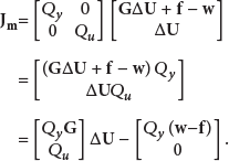
To minimize the cost function in (41), the solution of the algebraic equation (the control action) is derived as

\begin{matrix} [\begin{bmatrix} Q_{y} G \\ Q_{u} \end{bmatrix}] Δ U - [\begin{bmatrix} Q_{y} (w - f) \\ 0 \end{bmatrix}] = 0 . \end{matrix}

(42)

Equation (42) is further presented as follows:

\begin{matrix} \bar{A} Δ U = \bar{b}, \end{matrix}

(43)

where

\begin{matrix} \bar{A} = [\begin{bmatrix} Q_{y} G \\ Q_{u} \end{bmatrix}], \bar{b} = [\begin{bmatrix} Q_{y} (w - f) \\ 0 \end{bmatrix}] . \end{matrix}

(44)

For solving (42), the QR decomposition [21] method based on the Householder algorithm [22, 23] is used to decompose matrix $\bar{A}$ as

\begin{matrix} \bar{A} = Q R, \end{matrix}

(45)

where R is an upper triangular matrix and Q is an orthogonal matrix as

\begin{matrix} R = H_{N} H_{N - 1} {\dots H}_{1} \bar{A}, \\ Q = H_{1} H_{2} {\dots H}_{N - 1} \\ Q^{T} Q = {[H_{1} H_{2} {\dots H}_{N - 1}]}^{T} [H_{1} H_{2} {\dots H}_{N - 1}] = I, \end{matrix}

(46)

where

H_{i} (i = 1,2, \dots, N)

is a Householder matrix.

Considering (45), the solution of least squares in (43) is

\begin{matrix} {\bar{A}}^{T} (\bar{b} - \bar{A} Δ U) = 0 ⟹ R^{T} Q^{T} (\bar{b} - \bar{A} Δ U) = 0 \end{matrix}

(47)

Q^{T} \bar{A} = Q^{T} Q R = R

The preceding Equation (47) is rewritten as

\begin{array}{l} R^{T} Q^{T} (\bar{b} - \bar{A} Δ U) = 0 \\ ⟹ R^{T} (Q^{T} \bar{b} - Q^{T} \bar{A} Δ U) = 0 \\ ⟹ R^{T} (Q^{T} \bar{b} - R Δ U) = 0 . \end{array}

(48)

Thus, the control signal is obtained as

\begin{array}{l} Q^{T} \bar{b} = R Δ U ⟹ Δ U = {R^{- 1} Q}^{T} \bar{b} \\ ⟹ Δ U = {R^{- 1} Q}^{T} [\begin{bmatrix} Q_{y} (w - f) \\ 0 \end{bmatrix}] . \end{array}

(49)

Obtained vector $Δ U$ represents the control signal for the whole predictive horizon N , and the actual control signal sent to plant is the first element in (49).

2.4. State Estimator

Consider the system in state space which is presented in (27) as follows:

\begin{matrix} x (k + 1) = A x (k) + B u (k) + Π ω (k) \\ y (k) = C x (k) + ν (k), \end{matrix}

(50)

where ω and ν are sequences of white Gaussian noise with zero mean with known covariance as

\begin{matrix} E {ω (k)} = E {ν (k)} = 0 . \end{matrix}

(51)

The joint covariance matrix is

\begin{matrix} E {[\begin{bmatrix} ω (k) \\ ν (k) \end{bmatrix}] [\begin{bmatrix} ω^{T} (k) & ν^{T} (k) \end{bmatrix}]} = [\begin{bmatrix} Q_{0} & 0 \\ 0 & R_{0} \end{bmatrix}] . \end{matrix}

(52)

The initial state $x_{0}$ of a Gaussian random vector with mean presents i as

\begin{matrix} E {x_{0}} = {\hat{x}}_{0} . \end{matrix}

(53)

The covariance matrix is given by

\begin{matrix} E {(x_{0} {- \hat{x}}_{0}) {(x_{0} {- \hat{x}}_{0})}^{T}} = Σ_{0} . \end{matrix}

(54)

The conditional probability density functions (pdf) represent the Gaussian pdf as

\begin{matrix} 𝒫 (x (k)) ~ 𝒩 (\hat{x} (k), P (k)), \end{matrix}

(55)

where the state estimate

\hat{x} (k)

and the covariance matrix

P (k)

are presented as

\begin{matrix} \hat{x} (k) = E {x (k)} \\ P (k) = E {(x (k) - \hat{x} (k)) {(x (k) - \hat{x} (k))}^{T}} . \end{matrix}

(56)

Considering (55), the filtering cycle states at the instant $k + 1$ are presented as

\begin{matrix} 𝒫 (x (k + 1)) ~ 𝒩 (\hat{x} (k + 1), P (k + 1)), \end{matrix}

(57)

where

\begin{array}{l} \hat{x} (k + 1) = E {x (k + 1)} \\ P (k + 1) = E {(x (k + 1) - \hat{x} (k + 1)) \\ {\times (x (k + 1) - \hat{x} (k + 1))}^{T}} . \end{array}

(58)

The Gaussian pdf is characterized by the mean and covariance matrix. Considering (27) by applying the mean value operator which is presented as

\begin{matrix} E {x (k + 1)} = A \cdot E {x (k)} + B \cdot E {u (k)} + Π \cdot E {ω (k)} . \end{matrix}

(59)

From (55) and (57), the ω with zero mean is obtained as

\begin{matrix} \hat{x} (k + 1) = A \hat{x} (k) + B u (k) . \end{matrix}

(60)

The prediction error is defined as

\begin{matrix} \tilde{x} (k + 1) = x (k + 1) - \hat{x} (k + 1), \end{matrix}

(61)

which is replaced in expression of $x (k + 1)$ and $\hat{x} (k + 1)$ . Equation (61) is rewritten as

\begin{array}{l} \tilde{x} (k + 1) = A x (k) + B u (k) + Π ω (k) \\ - A \hat{x} (k) - B u (k) = A \tilde{x} (k) + Π ω (k), \end{array}

(62)

where the filtering error is

\tilde{x} (k) = x (k) - \hat{x} (k)

Equation (59) is rewritten as follows:

\begin{matrix} E {(\tilde{x} (k + 1)) {(\tilde{x} (k + 1))}^{T}} = A {E {\tilde{x} (k)} A}^{T} + Π Q_{0} Π^{T} . \end{matrix}

(63)

From (63), the notations in (56) and (58) result in

\begin{matrix} P (k + 1) = A P (k) A^{T} + Π Q_{0} Π^{T} . \end{matrix}

(64)

The predictive estimated states of the system and the associated covariance matrix in (60) and (64) correspond to the optimal system state at the time instant $k + 1$ before making observation at time instant k. The predicted measurement with a Gaussian pdf is given by

\begin{matrix} \hat{y} (k + 1) = E {y (k + 1)} = C \hat{x} (k + 1) . \end{matrix}

(65)

The measurement prediction error $\tilde{y} (k + 1) = y (k + 1) - \hat{y} (k + 1)$ is rewritten by replacing the y and $\hat{y}$ as

\begin{matrix} \tilde{y} (k + 1) = C \hat{x} (k + 1) + ν (k) . \end{matrix}

(66)

Considering (66), the covariance matrix is obtained as

\begin{matrix} P_{\tilde{y}} (k + 1) = C P (k + 1) C^{T} + R_{0} . \end{matrix}

(67)

Multiply $x (k + 1)$ on both sides of transpose in (66) as

\begin{array}{l} x (k + 1) {\tilde{y}}^{T} (k + 1) = x (k + 1) C^{T} {\hat{x}}^{T} (k + 1) \\ + x (k + 1) ν^{T} (k) . \end{array}

(68)

Consider $E {x (k + 1) {\tilde{y}}^{T} (k + 1)} = P (k + 1) C^{T}$ and evaluate the estimate state $\hat{x}$ at time instant $k + 1$ as

\begin{array}{l} \hat{x} (k + 1) = E {x (k + 1)} \\ + E {x (k + 1), {\tilde{y}}^{T} (k + 1) {P_{\tilde{y}}}^{- 1} (k + 1) \tilde{y} (k + 1)} . \end{array}

(69)

The optimal estimator to compute the state is based on a Kalman filter. The j-step ahead system output presented in (34) is

\begin{matrix} y (k + j) = {C A}^{j} \hat{x} (k) + \sum_{i = 1}^{j} {C A}^{i - 1} B Δ u (k + j - i) . \end{matrix}

(70)

In (69), the estimation of the state vector $\hat{x}$ is obtained by the Kalman filter as

\begin{array}{l} \hat{x} (k) = A \hat{x} (k - 1) + B Δ u (k - 1) + K_{g} (k) \\ \times {y (k) - C [A \hat{x} (k - 1) + B Δ u (k - 1)]}, \end{array}

(71)

where

K_{g}

is Kalman filter gain matrix represented in (72) to adapt the estimation of model states to measure the outputs from controlled system. Consider

\begin{matrix} K_{g} (k) = P (k - 1) C^{T} {[C P (k - 1) C^{T} + R]}^{- 1}, \end{matrix}

(72)

where the updated error covariance is

P (k) = [I - K_{g} (k) C] P (k - 1)

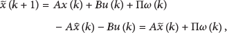
Figure 2 shows the block diagram of the state estimator using Kalman filter to provide the estimate state for GPC. The Kalman filter is linear, discrete time, and finite dimension. The filter gain is independent of the system outputs. The error covariance and the filter gain are calculated before the filter is executed.

Figure 2

State estimator with Kalman filter.

3. Result

3.1. GPC Implementation in WiNCS

Figure 3 shows the setup for the proposed GPC controller with Kalman state estimator implemented; control and sensor signals are encapsulated into packets to transmit in a wireless network environment emulated by NS2 (see the Appendix) under the WiNCS client/server architecture (IEEE 802.11b protocol) provided by PiccSIM (see the Appendix).

Figure 3

Experiment setup: (a) hardware and (b) software.

The simulation architecture is illustrated in Figure 4. The control system is in the server. The sensor, actuator, and plant are in the client under an emulated IEEE 802.11b wireless network.

Figure 4

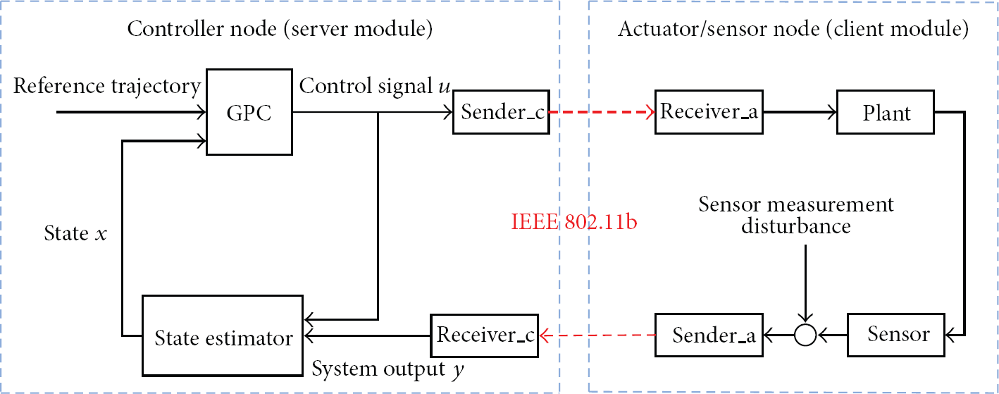
Structure of WiNCS.

3.1.1. Controller Node

The controller node in server module includes GPC controller, Kalman state estimator, sender, and receiver as shown in Figure 5. The square wave (period: 15 seconds, peaks: 1, and duration: from 0 to 100 seconds) is applied as the controller input.

Figure 5

Simulation architecture of controller node.

3.1.2. Actuator/Sensor Node

The actuator/sensor node in the client module includes actuator, plant, sensor, sender, and receiver as shown in Figure 6. A white noise is applied as the disturbance to sensor measurement. The discrete state-space plant model is given by

\begin{matrix} x (k + 1) = [\begin{bmatrix} - 0.0304 & - 0.0998 \\ 0.1058 & 0.3476 \end{bmatrix}] x (k) + [\begin{bmatrix} 0.2116 \\ 1.3834 \end{bmatrix}] u (k) \\ y (k) = [\begin{bmatrix} 0 & 15.858 \end{bmatrix}] x (k) . \end{matrix}

(73)

Figure 6

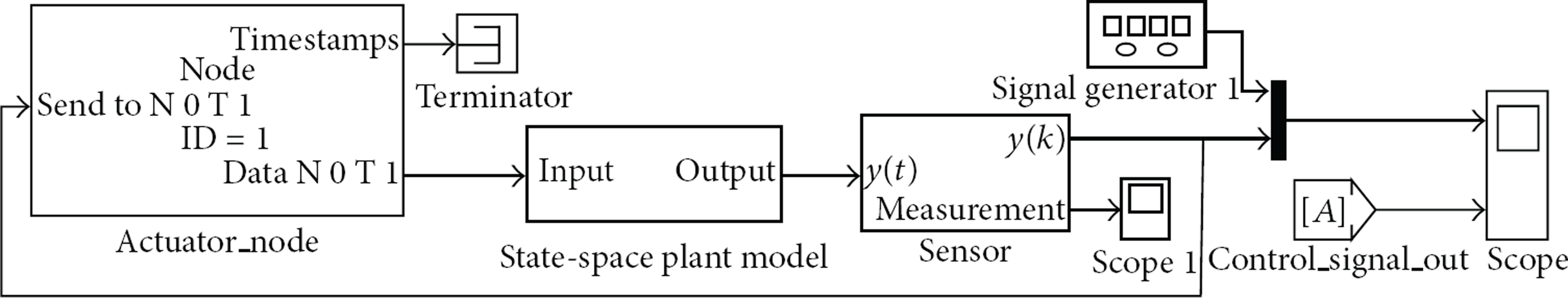
Simulation architecture of actuator/sensor node.

3.2. Latency and Throughput on Actual Wireless Network Environment

The performance of the networked data acquisition system for an actual small UAV (CoaX helicopter) is evaluated with the topology in Figure 7. The UAV sends images to a ground-based computer where the data is processed, and control packages are sent back to the UAV. Latency and throughput of the system are determined with the hrPing utility and the Interprocess Communication (IPC) library (see the Appendix).

Figure 7

Topology of the wireless network for performance testing.

Experiments were performed in two different indoor environments. The first is a room with a square ground plane and the second is a long corridor as shown in Figures 8 and 9. The line of sight connection of the transmission is uninterrupted by massive structures like concrete walls at all times.

Figure 8

Square-shaped room for wireless network parameter measurements.

Figure 9

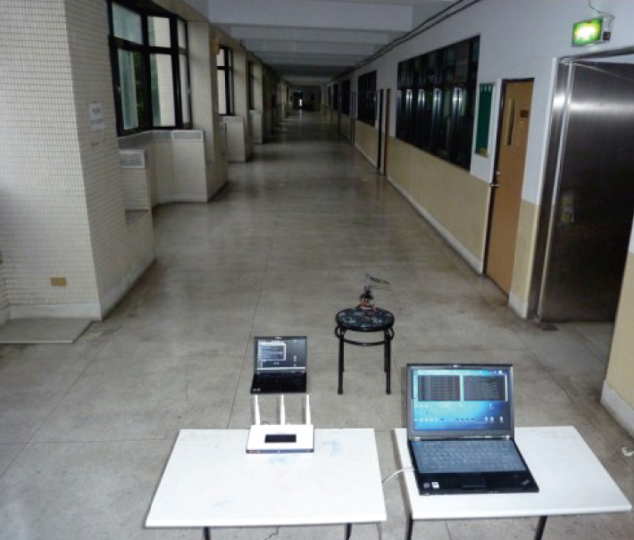
Long corridor for wireless network parameter measurements.

The latency and throughput are tested for several distances between the CoaX helicopter and the stationary wireless router under two standards (IEEE 802.11 g and IEEE 802.11n). IEEE 802.11n provides longer range and higher throughput. The throughput of the wireless connection is determined for data packet sizes between 1 kB and 256 kB. The transfer rate for smaller packets is lower because the overhead of the transmission is dominant.

3.2.1. Laboratory Environment

The average latency of the IEEE 802.11 g connection (Figure 10) is constantly very low, and also the maximum values are stable over the whole distance range. Figure 11 shows the measurements for the connection conforming IEEE 802.11n. The mean latency is slightly higher, but the maximum latency does not significantly exceed the results of the previous measurements.

Figure 10

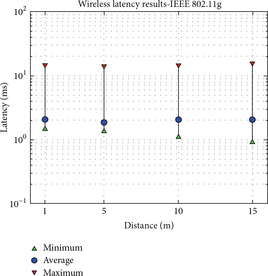
Latency measurements in room—IEEE 802.11 g.

Figure 11

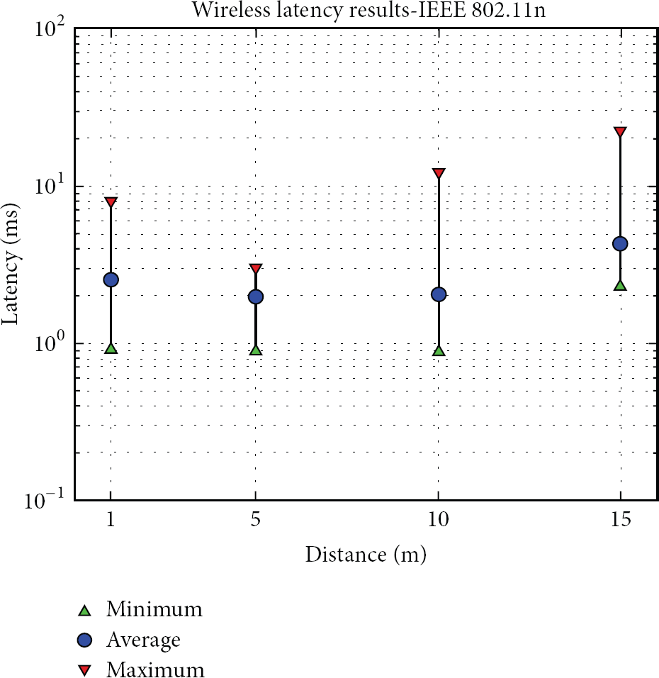
Latency measurements in room—IEEE 802.11n.

The throughput of the connection with the CoaX helicopter (IEEE 802.11 g), shown in Figure 12, is practically independent of the distance in this environment. In the measurements with the IEEE 802.11n connection (Figure 13), the throughput decreases with longer distance for bigger data packets.

Figure 12

Throughput measurements in room—IEEE 802.11 g.

Figure 13

Throughput measurements in room—IEEE 802.11n.

3.2.2. Corridor Environment

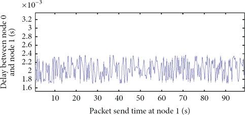
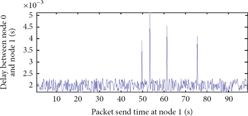
The measurements are taken in the long corridor at distances from 10 to 70 meters. The latency of the connection with the CoaX helicopter (IEEE 802.11 g) is illustrated in Figure 14. The results show that the average latency is very low at around 1.2 ms, which is close to the minimum value. The worst case of the latency in the measurements is 20 ms. The measurements of a connection with the recently introduced standard IEEE 802.11n are shown in Figure 15. The average latency for distances from 30 meters and higher is low at around 1.2 ms. In close distance, however, the mean latency rises to 6.5 ms and the maximum value of 100 ms is comparatively high.

Figure 14

Latency measurements in corridor—IEEE 802.11 g.

Figure 15

Latency measurements in corridor—IEEE 802.11n.

The results for the throughput of the connection with IEEE 802.11 g are depicted in Figure 16. The throughput decreases with rising distance up to 60 meters; however, the measurement for 70 meters gave a higher value. As expected, the connection with IEEE 802.11n achieved significantly higher transfer rates. The data in Figure 17 shows that the throughput decreases as the distance is increased.

Figure 16

Throughput measurements in corridor—IEEE 802.11 g.

Figure 17

Throughput measurements in corridor—IEEE 802.11n.

3.3. System Response with Random Delay and Packets Loss

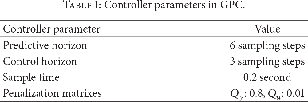
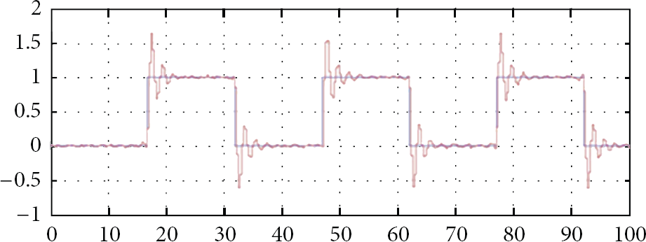
This experiment is to evaluate the capability of the proposed GPC with Kalman state estimator approach for compensating the random time delay in NCS. The random delay model is adopted to validate the GPC capability of compensating the delays. The system response is shown in Figure 18 with the random delay between 160 ms and 200 ms. The GPC parameters are listed in Table 1. The system response is stable but with the higher overshoot and the longer settling time. When the delay time closes to the sample time, the system response occurs with highly jitter.

Table 1

Controller parameters in GPC.

Controller parameter	Value
Predictive horizon	6 sampling steps
Control horizon	3 sampling steps
Sample time	0.2 second
Penalization matrixes	$Q_{y}$ : 0.8, $Q_{u}$ : 0.01

Figure 18

System response with random delay between 160 ms and 200 ms.

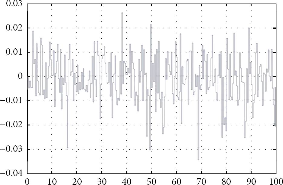
The packet loss phenomenon is emulated by a switch with various packet loss rates. Figure 19 shows the system response with random delay between 120 ms and 160 ms and packets loss rate 5%. The higher packet loss rate causes the higher jitter of the system response (unstable).

Figure 19

System response with random delay between 120 ms and 160 ms and packets loss rate 5%. x-axis: time (sec.) and y-axis: magnitude.

3.4. System Response with Network-Induced Delay in NS2

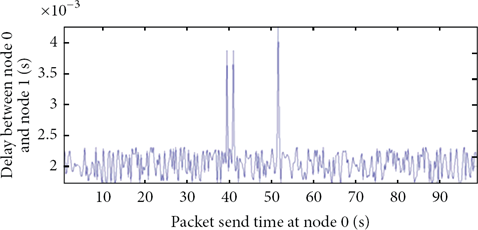
The network-induced delay is generated by NS2 to evaluate if the system can follow the reference trajectory. Figure 20 shows the system response. Figures 21, 22, and 23 show the controller-to-actuator delay, sensor-to-controller delay, and sensor disturbance measurement, respectively. The simulation information is listed in Table 2. All of the packets were successfully transmitted without dropped packets. The system response successfully follows the reference trajectory as shown in Figure 20.

Table 2

Simulation information of nodes with sample time 0.4 sec.

Simulation specification	Value
Number of generated packets	500
Number of sent packets	500
Average packet size	43.4973
Number of sent bytes	32960

Figure 20

WiNCS response with sample time 0.4 sec. x-axis: time (sec.) and y-axis: magnitude.

Figure 21

Controller-to-actuator delay with sample time 0.4 sec. x-axis: time (sec.) and y-axis: magnitude.

Figure 22

Sensor-to-controller delay with sample time 0.4 sec. x-axis: time (sec.) and y-axis: magnitude.

Figure 23

Sensor noise measurement with sample time 0.4 sec. x-axis: time (sec.) and y-axis: magnitude.

Figure 24 shows the system response with sample time 0.3 sec. Figures 25, 26, and 27 show the controller-to-actuator delay, sensor-to-controller delay, and sensor disturbance measurement, respectively. The simulation information is listed in Table 3. The system is stable but with higher overshoot and the longer settling time. Different sample times affect the system performance. When the system is with the short sample time, the sender must generate more data packets. It might raise the packets loss rate and shorten the predictive horizon which might cause system unstablility.

Table 3

Simulation information of nodes with sample time 0.3 sec.

Simulation information	Value
Number of generated packets	668
Number of sent packets	668
Average packet size	43.7701
Number of sent bytes	44048

Figure 24

WiNCS response with sample time 0.3 sec. x-axis: time (sec.) and y-axis: magnitude.

Figure 25

Controller-to-actuator delay with sample time 0.3 sec. x-axis: time (sec.) and y-axis: magnitude.

Figure 26

Sensor-to-controller delay with sample time 0.3 sec. x-axis: time (sec.) and y-axis: magnitude.

Figure 27

Sensor noise measurement with sample time 0.3 sec. x-axis: time (sec.) and y-axis: magnitude.

Figure 28 shows the system response with sample time 0.2 sec. Figures 29, 30, and 31 show the controller-to-actuator delay, sensor-to-controller delay, and sensor disturbance measurement, respectively. The system response is highly jitter and with longer settling time. The simulation information is listed in Table 4. The system response already cannot follow the reference trajectory.

Table 4

Simulation information of nodes with sample time 0.2 sec.

Simulation information	Value
Number of generated packets	1002
Number of sent packets	1000
Number of dropped packets	2
Average packet size	44.1737
Number of sent bytes	65920
Number of dropped bytes	132

Figure 28

WiNCS response with sample time 0.2 sec. x-axis: time (sec.) and y-axis: magnitude.

Figure 29

Controller-to-actuator delay with sample time 0.2 sec. x-axis: time (sec.) and y-axis: magnitude.

Figure 30

Sensor-to-controller delay with sample time 0.2 sec. x-axis: time (sec.) and y-axis: magnitude.

Figure 31

Sensor noise measurement with sample time 0.2 sec. x-axis: time (sec.) and y-axis: magnitude.

Figure 32 shows the system response with sample time 0.1 sec. The shorter sample time cause system unstable in WiNCS due to it shorten the predictive horizon.

Figure 32

WiNCS response with sample time 0.1 sec. x-axis: time (sec.) and y-axis: magnitude.

4. Discussion

The WiNCS is implemented and evaluated with random delay, network-induced delay, and packets loss implementation by an analytical model and NS2. Result shows that the system response could follow the reference trajectory with the condition of the time delay under 160 ms and sample time 0.2 s. The system response jittered when packet loss rate exceeded 10%.

The WiNCS is also simulated by NS2 with AOVD protocol. Result shows the system response with sample time = 0.4 sec. and number of transmission data packets = 500 and sample time = 0.3 sec. number of transmission data packets = 668 can follow the reference trajectory. The system response with sample time = 0.2 sec, number of transmission data packets = 1002, and number of packets loss = 2 has high jitter. The different sample times have various numbers of transmission data packets. The larger the number of transmission data packets is, the easier the packets loss occurs.

It is easier to evaluate the performance of GPC in WiNCS when it is simulated via a model because the condition of random delay and packets loss rate can be controlled. WiNCS implemented in NS2 is closer to actual wireless network; therefore, the distance between control node and actuator/sensor node affects the network-induced delay and packets loss. This causes GPC performance to be difficult to analyse. The parameter in NS2 needs to be reestimated when being in the various wireless coverage environments. This also affects the simulation results when GPC is implemented in WiNCS.

The wireless networked control system results suggest that the latency is not directly related to the distance between sender and receiver. The mean values of the measurements are adequate for a closed-loop control system; however, the maximum values might have to be considered depending on the application. One reason for latency is the property that different wireless networks share the same frequency channel. Therefore, the density of wireless networks and the rate of traffic in close vicinity to the measurement setup determine the latency of the connection.

The throughput of the wireless connection according to standard IEEE 802.11 g is sufficient to transmit compressed images of size 320 × 240 at a rate of 30 frames per second up to a distance of 70 meters. The connection with the faster IEEE 802.11n standard allows transmitting the same images with smaller time delay or images with higher resolution at the same rate.

The measurements suggest that the concept of the wireless networked control system is applicable to autonomous navigation of small UAVs. The latency in a controlled environment is very low and does not inhibit real-time closed-loop control applications. The throughput of either standard IEEE 802.11 g or IEEE 802.11n is sufficient for transmitting compressed images of adequate resolution at a rate of 30 frames per second; however, the standard IEEE 802.11n is preferable for better performance.

The ideal environment for the wireless networked control system approach would be a closed room with strong walls to shield against interference from other networks. The limitations of the proposed system are the high sensitivity to interference from other wireless sources and the necessity of a line of sight connection without massive obstacles like concrete walls.

5. Conclusion

This paper proposed the GPC controller with Kalman state estimator in WiNCS based on PiccSIM platform. The packets are exchanged between the controller node and actuator/sensor node via wireless network IEEE 802.11b which is emulated by NS2. Although network-induced delay characteristics in the wireless communication network are difficult to model, this paper describes the main problems which might induce the time delay.

This paper simplifies complex architectures in the wireless communication network for analysis proposed with WiNCS which is simulated in NS2 using the two-ray ground model. First, this study implements WiNCS with the random delay to verify GPC controller capability with the Kalman state estimator to cope with time delay. Then, WiNCS is implemented with NS2 to present the effect of different sample times in the predictive horizon; that is, system performance decreases when sample time decreases. When WiNCS is implemented with the sample time of 0.2 seconds, the packets start to drop, affecting the system performance.

We also propose the basic WiNCS simulation on a low-level control system. Realizing WiNCS requires not only improving the control algorithm to compensate for time delay, but also improving wireless communication performance. The time delay occurred when the packets are exchanged in the network. The algorithm for optimizing network performance communication is also important. This paper proposes the GPC algorithm for compensating time delay which focuses on improving control algorithm. In future, it is required to have further integration of the automation and control and network communication for realizing WiNCS.

The concept for a wireless networked control system was evaluated with latency and throughput measurements in different environments. The experiment setup conforming to the IEEE 802.11n standard achieves an average latency of 1.3 ms and a data throughput of 3.000 kB/s up to a distance of 70 m. The results demonstrate the feasibility of real-time closed-loop navigation control with the proposed concept.

The only significant limitations of the wireless networked control concept are the relatively short range of the wireless connections and the sensitivity to congest with other wireless devices. However, neither of them inhibits the effectiveness of the concept in the designated application to research in a controlled environment.

Modeling the network-induced delay and packets loss is extremely difficult. Although the NS2 provides the simulated communication network environment, it still simplifies the network condition comparing with real network devices. In this paper, the GPC implemented in WiNCS was verifying that it is a feasibility study.

In future work, a network estimator must be implemented and measure the network-induced delay and round trip time delay for tuning the controller parameters for increasing the performance of WiNCS. In addition, the soft computing technique (e.g., artificial neural network) can be applied to the predictive control algorithm to minimize the predictive error or tune the parameters of network estimator.

Footnotes

Appendix

References

Zhang

Branicky

M. S.

Phillips

S. M.

Stability of networked control systems

IEEE Control Systems Magazine 2001 21 1 84 99

2-s2.0-0034831393

10.1109/37.898794

Tipsuwan

Chow

M.-Y.

Control methodologies in networked control systems

Control Engineering Practice 2003 11 10 1099 1111

2-s2.0-0141924276

10.1016/S0967-0661(03)00036-4

Wang

F.-Y.

Liu

Networked Control Systems:Theory and Applications 2008

London, UK

Springer

Leung

W.-L. D.

Vanijjirattikhan

Richards

Ayhan

Chow

M.-Y.

Intelligent space with time sensitive applications

Proceedings of the IEEE/ASME International Conference on Advanced Intelligent Mechatronics (AIM '05)

July 2005

1413 1418

2-s2.0-27644453165

Walsh

G. C.

Bushnell

L. G.

Stability analysis of networked control systems

IEEE Transactions on Control Systems Technology 2002 10 3 438 446

2-s2.0-0036575409

10.1109/87.998034

Walsh

G. C.

Beldiman

Bushnell

Asymptotic behavior of networked control systems

Proceedings of the IEEE International Conference on Control Applications (CCA '99)

August 1999

1448 1453

2-s2.0-0033320104

Chow

M.-Y.

Tipsuwan

Gain adaptation of networked DC motor controllers based on QOS variations

IEEE Transactions on Industrial Electronics 2003 50 5 936 943

2-s2.0-0141952875

10.1109/TIE.2003.817576

Zhang

Shi

Chen

Huang

A new method for stabilization of networked control systems with random delays

IEEE Transactions on Automatic Control 2005 50 8 1177 1181

2-s2.0-26244435112

10.1109/TAC.2005.852550

Montestruque

L. A.

Antsaklis

Stability of model-based networked control systems with time-varying transmission times

IEEE Transactions on Automatic Control 2004 49 9 1562 1572

2-s2.0-4644285812

10.1109/TAC.2004.834107

10.

Yue

Han

Q.-L.

Peng

State feedback controller design of networked control systems

IEEE Transactions on Circuits and Systems II 2004 51 11 640 644

2-s2.0-9744285848

10.1109/TCSII.2004.836043

11.

Beldiman

Walsh

G. C.

Bushnell

Predictors for networked control systems

Proceedings of the American Control Conference

June 2000

2347 2351

2-s2.0-0034542676

12.

Aiguo

Dongqing

Jin

Application of generalized predictive control with neural network error correction in networked control system

Proceedings of the 5th World Congress on Intelligent Control and Automation (WCICA '04)

2004

1386 1390

13.

Dejun

Lei

Guanzhong

Research on generalized predictive control algorithm of networked control system

Proceedings of the 25th Chinese Control Conference (CCC '06)

August 2006

119 122

2-s2.0-37349118647

10.1109/CHICC.2006.280603

14.

Tang

P. L.

de Silva

C. W.

Compensation for transmission delays in an ethernet-based control network using variable-horizon predictive control

IEEE Transactions on Control Systems Technology 2006 14 4 707 718

2-s2.0-33745623949

10.1109/TCST.2006.876640

15.

Witrant

Park

P. G.

Johansson

Fischione

Johansson

K. H.

Predictive control over wireless multi-hop networks

Proceedings of the 16th IEEE International Conference on Control Applications (CCA '07)

October 2007

Singapore

1037 1042

2-s2.0-43049165825

10.1109/CCA.2007.4389370

16.

Clarke

D. W.

Mohtadi

Tuffs

P. S.

Generalized predictive control. Part I. The basic algorithm

Automatica 1987 23 2 137 148

2-s2.0-0023310961

17.

Camacho

C. B. E. F.

Model Predictive Control 2004

Berlin, Germany

Springer

18.

Clarke

D. W.

Mohtadi

Tuffs

P. S.

Generalized predictive control. Part II. Extensions and interpretations

Automatica 1987 23 2 149 160

2-s2.0-0023311208

19.

Soloway

Shi

Kelkar

GPC-Based Stable Reconfigurable Control 2004

NASA Ames Research Center

20.

Belda

Bohm

Range-space predictive control for optimal robot motion

International Journal of Circuits, Systems and Signal Processing 2007 1 1

21.

Press

W. H.

Teukolsky

S. A.

Vetterling

W. T.

Flannery

B. P.

Numerical Recipes: The Art of Scientific Computing 2007 3rd

Cambridge, UK

Cambridge University Press

22.

Golub

G. H.

Loan

C. F. V.

Matrix Computations 1996 3rd

Baltimore, Md, USA

Johns Hopkins University

23.

Yang

W. Y.

Cao

Chung

T. S.

Morris

Applied Numerical Methods Using MATLAB 2005

Hoboken, NJ, USA

John Wiley & Sons

Generalized Predictive Control in a Wireless Networked Control System

Abstract

1. Introduction

2. Method

2.1. Formulation of GPC

2.2. GPC Control Strategy

2.3. GPC in State-Space Formulation

2.4. State Estimator

3. Result

3.1. GPC Implementation in WiNCS

3.1.1. Controller Node

3.1.2. Actuator/Sensor Node

3.2. Latency and Throughput on Actual Wireless Network Environment

3.2.1. Laboratory Environment

3.2.2. Corridor Environment

3.3. System Response with Random Delay and Packets Loss

3.4. System Response with Network-Induced Delay in NS2

4. Discussion

5. Conclusion

Footnotes

Appendix

References