Variable-Weighted Grayscale Centroiding and Accuracy Evaluating

Abstract

Grayscale-weighted centroiding weights the pixel intensity to estimate the center of a circular image region such as a photogrammetric target or a star image. This is easy to realize with good robustness; however, locating accuracy varies with weight. There is no conclusion as to the relationship between weight and centroiding accuracy. To find this relationship and thus acquire the highest achievable accuracy of centroiding, one must first derive the general model of centroiding as follows. (1) Set weighting as a function that includes the grayscale intensity of each pixel and two undetermined parameters α and β. The centers were calculated from the new weights. (2) Design an accuracy evaluation method for centroiding based on a virtual straight-line target to obtain the accuracy of centroiding with various parameters. With these parameter values and accuracy records, the accuracy-parameter curve can be fitted. In the end, simulations and experiments are conducted to prove the accuracy improvement of this variable-weighted grayscale centroiding compared with traditional centroiding. The experimental result shows that the parameter α contributes significantly to accuracy improvement. When α = 1.5, locating accuracy is 1/170 pixels. Compared to centroiding and squared centroiding, the new locating method has a 14.3% and 10.6% accuracy improvement indicating that it improves locating accuracy effectively.

1. Introduction

Large-scale photogrammetry is mainly applied to precise locating and measuring in automobile, aircraft, shipbuilding, and other large-scale industrial manufacturing and assembling; surface measurements of satellite antennas and radio telescopes; and deformation measurements in load tests of large parts [1, 2]. Unlike small-scale measurement [3], large-scale photogrammetry is always used to measure large objects; it requires extremely favorable relative precision to ensure high accuracy. As the source data of photogrammetric metrology, the accuracy of photogrammetry is greatly affected by the determination of the target image coordinates. Target image locating accuracy is affected by environmental conditions, target characteristics, imaging system performance, and the locating algorithm, where environmental conditions can be optimized according to specific requirements. Since Brown applied retro-reflective target (RRT) to photogrammetry, target image quality has been greatly improved. It is easy to obtain a quasibinary image. Currently the limitation of locating accuracy is mainly caused by imaging system performance and the locating algorithm.

Digital imaging systems have great advantages over film imaging systems, and they are gradually replacing film imaging systems. A digital imaging system performance index includes the lens modulation transfer function, the resolution of the charge-coupled device (CCD, there are also other imaging sensors, for example, CMOS, but CCDs are most commonly used in digital close-range photogrammetry) resolution, the photoelectric conversion efficiency, and electrostatic noise. Nowadays, CCD resolution is the major factor that limits locating accuracy. Limited by the manufacturing process, digital cameras have resolutions of several megapixels when it was newly applied to photogrammetry, and it was only half size of the 135 film. Until now, the size of the CCD in most advanced digital camera backs on the market is generally about 50 mm × 40 mm. The resolution varies from 50 to 80 megapixels, while the film camera CRC-1 which was designed by Brown in 1984 has a film format of 230 mm × 230 mm with an equivalent pixel size of 3.1 μm × 2.5 μm [4]. That means that film has an equivalent resolution of 6 giga pixels, which is far higher than CCD cameras. This results in the fact that the highest accuracy the large field digital photogrammetry products can reach is about 1/200,000, which is lower than the film photogrammetry systems designed 20 years ago [5, 6]. Therefore, researchers turn to subpixel locating technology.

The proposed target image locating method can be divided into three main categories. The first is model fitting based on intensity distribution, such as Gaussian surface fitting. This method requires an intensity distribution model; however, it is difficult to model a facula precisely especially for large RRT, that may transfer or enlarge the error. The second is shape fitting based on target appearance, such as ellipse fitting. This method relies on the edge locating accuracy. It is more difficult to locate an edge precisely than the whole target image since there is less information. Moreover, the affine transformation distinguishes between the two centers in the image plane and the object space [7]. The third is weighted centroiding based on gray intensity weighting. This method calculates the whole target image and estimates its center as the gray intensity center. It has good robustness to noise, and the computing is simple. Locating accuracy differs as weights change with the form of a nonlinear function.

The two existing examples are centroiding and squared centroiding. Studies indicate that squared centroiding has superior accuracy [8]. But there is no evidence that squared grayscale weight has optimal accuracy for weighted centroid locating. This paper derives a general model of centroiding. The weight is set as a function of pixel grayscale intensity of two undetermined parameters α and β, and then an analysis is conducted to prove that there is a set of α and β providing the highest accuracy location for grayscale-weighted centroiding. Then an accuracy evaluating method is designed to obtain accurate centroiding with various parameter values. With these parameter values and accuracy records, the accuracy-parameter curve can be fitted. Meanwhile the optimal values for α and β are obtained.

2. Variable-Weighted Grayscale Centroiding

2.1. Retro-Reflective Target (RRT)

As already mentioned, applying RRT to photogrammetry has vastly contributed to the development of photogrammetry. RRT materials can be classified as glass beads or microprisms according to their basic structure. Considering the production process, costs, and reflection symmetry properties, the glass bead RRT is used most commonly. Glass bead is the basic reflective element (Figure 1 (a)). The glass beads are deposited onto a reflective layer. The incident light is refracted through the glass beads, focused onto reflecting layer behind the glass beads, and then returned to the incident side through reflection and refraction (Figure 1 (b)) [9]. To make sure that the whole reflecting surface of RRT is uniform, the size of glass beads must be small enough, typically 10–30 μm. To achieve good retro-reflective performance, the refractive index of the glass beads is generally between 1.9 and 2.2.

Figure 1:

RRT structure and light path.

Due to the retro-reflectivity of RRT, the reflected light intensity in the light source direction is up to hundreds of even thousands of times that of a diffuse target [10]. Thus, it is easy to obtain a quasibinary image with a separated target image and background. This helps in target recognition and extraction as well as in high-precision locating (Figure 2).

Figure 2:

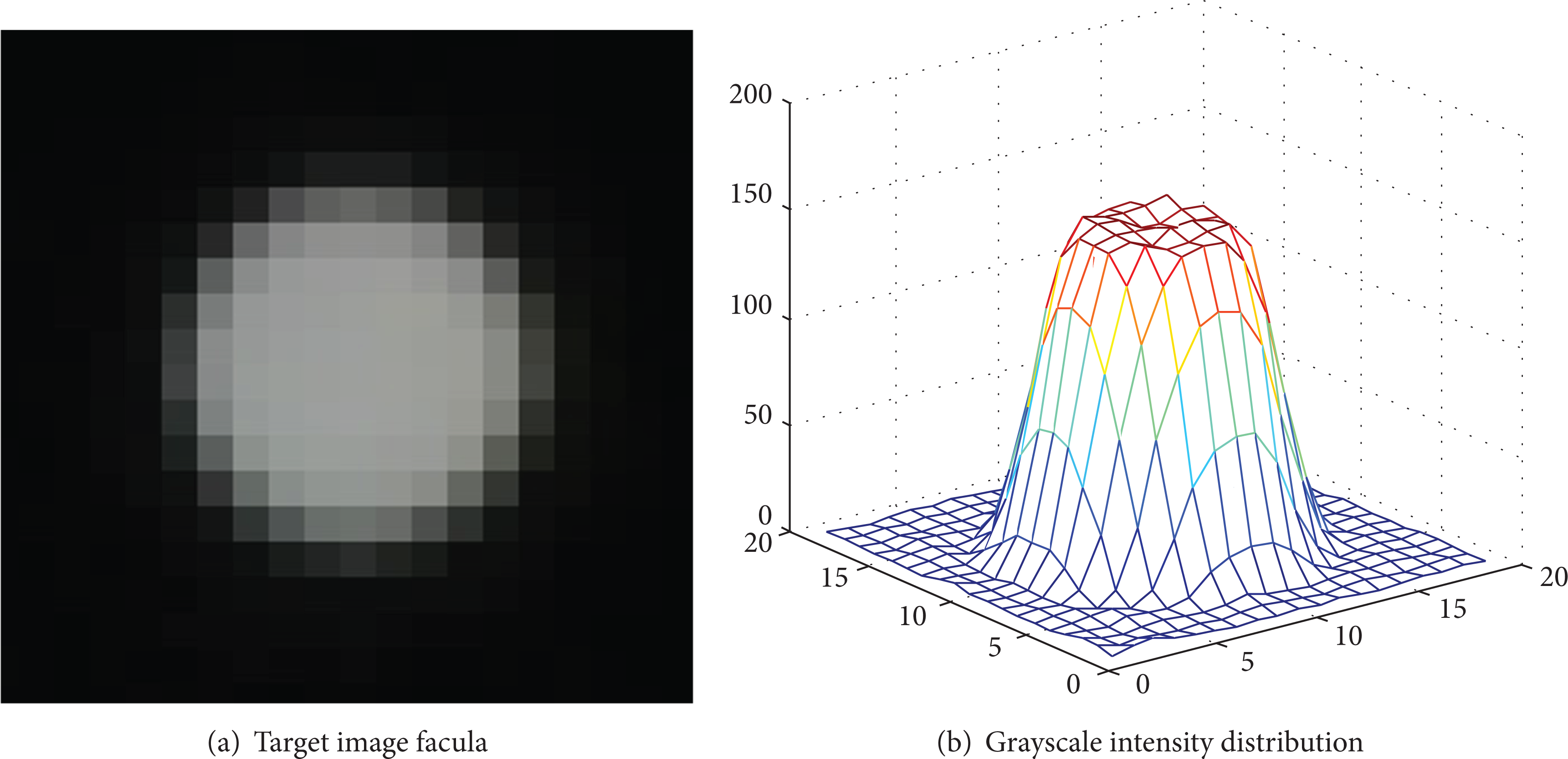
Image of an RRT.

RRT's quasibinary image feature is effective for noise suppression, and, because the entire region of the target image is calculated, random noise plays a tiny role in grayscale-weighted centroiding.

2.2. Variable Grayscale-Weighted Centroiding

Grayscale-weighted locating methods typically include the following three specific methods: grayscale centroiding, grayscale centroiding with threshold, and squared grayscale-weighted centroiding.

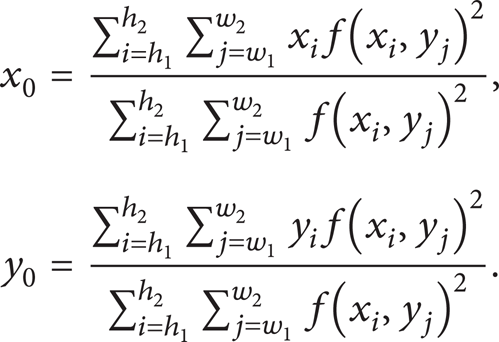
Grayscale centroiding is given by

$\begin{array}{c}{x}_{\mathrm{0}}=\frac{{\sum }_{i=h_{\mathrm{1}}}^{h_{\mathrm{2}}}{\sum }_{j=w_{\mathrm{1}}}^{w_{\mathrm{2}}}{x}_{i}f\left(x_i,y_j\right)}{{\sum }_{i=h_{\mathrm{1}}}^{h_{\mathrm{2}}}{\sum }_{j=w_{\mathrm{1}}}^{w_{\mathrm{2}}}f\left(x_i,y_j\right)},\\ y_{\mathrm{0}}=\frac{{\sum }_{i=h_{\mathrm{1}}}^{h_{\mathrm{2}}}{\sum }_{j=w_{\mathrm{1}}}^{w_{\mathrm{2}}}{y}_{i}f\left(x_i,y_j\right)}{{\sum }_{i=h_{\mathrm{1}}}^{h_{\mathrm{2}}}{\sum }_{j=w_{\mathrm{1}}}^{w_{\mathrm{2}}}f\left(x_i,y_j\right)},\end{array}$

(1)

where f(x _i , y _i ) is the grayscale intensity at coordinate (x _i , y _i ), x _i ∊ [w₁, w₂], y _j ∊ [h₁, h₂], and (x₀, y₀) is the calculated centroid.

Grayscale centroiding with threshold is given by

$\begin{array}{c}{x}_{\mathrm{0}}=\frac{{\sum }_{i=h_{\mathrm{1}}}^{h_{\mathrm{2}}}{\sum }_{j=w_{\mathrm{1}}}^{w_{\mathrm{2}}}{x}_i\left[f\left(x_i,y_j\right)-\text{th}\right]}{{\sum }_{i=h_{\mathrm{1}}}^{h_{\mathrm{2}}}{\sum }_{j=w_{\mathrm{1}}}^{w_{\mathrm{2}}}\left[f\left(x_i,y_j\right)-\text{th}\right]},\\ y_{\mathrm{0}}=\frac{{\sum }_{i=h_{\mathrm{1}}}^{h_{\mathrm{2}}}{\sum }_{j=w_{\mathrm{1}}}^{w_{\mathrm{2}}}{y}_i\left[f\left(x_i,y_j\right)-\text{th}\right]}{{\sum }_{i=h_{\mathrm{1}}}^{h_{\mathrm{2}}}{\sum }_{j=w_{\mathrm{1}}}^{w_{\mathrm{2}}}\left[f\left(x_i,y_j\right)-\text{th}\right]}.\end{array}$

(2)

Compared with grayscale centroid, this equation subtracts a constant th from the grayscale intensity. The value of th should be set to eliminate noise based on its expected value [8], particularly when the expected value is high.

Squared grayscale-weighted centroiding is as follows:

$\begin{array}{c}{x}_{\mathrm{0}}=\frac{{\sum }_{i=h_{\mathrm{1}}}^{h_{\mathrm{2}}}{\sum }_{j=w_{\mathrm{1}}}^{w_{\mathrm{2}}}{x}_{i}f{\left(x_i,y_j\right)}^{\mathrm{2}}}{{\sum }_{i=h_{\mathrm{1}}}^{h_{\mathrm{2}}}{\sum }_{j=w_{\mathrm{1}}}^{w_{\mathrm{2}}}f{\left(x_i,y_j\right)}^{\mathrm{2}}},\\ y_{\mathrm{0}}=\frac{{\sum }_{i=h_{\mathrm{1}}}^{h_{\mathrm{2}}}{\sum }_{j=w_{\mathrm{1}}}^{w_{\mathrm{2}}}{y}_{i}f{\left(x_i,y_j\right)}^{\mathrm{2}}}{{\sum }_{i=h_{\mathrm{1}}}^{h_{\mathrm{2}}}{\sum }_{j=w_{\mathrm{1}}}^{w_{\mathrm{2}}}f{\left(x_i,y_j\right)}^{\mathrm{2}}}.\end{array}$

(3)

This method weights the coordinate as a squared gray value, thereby changing the signal-to-noise ratio (SNR). Many studies have shown that this improves locating accuracy.

Based on the induction of the above grayscale centroid-locating algorithms, the general algorithm is derived. Let coordinate (x _i , y _i ) be weighted by ${[f(x_i,y_i)-\beta ]}^{\alpha }$ ; then

$\begin{array}{c}{x}_{\mathrm{0}}=\frac{{\sum }_{i=h_{\mathrm{1}}}^{h_{\mathrm{2}}}{\sum }_{j=w_{\mathrm{1}}}^{w_{\mathrm{2}}}{x}_i{\left[f\left(x_i,y_j\right)-\beta \right]}^{\alpha }}{{\sum }_{i=h_{\mathrm{1}}}^{h_{\mathrm{2}}}{\sum }_{j=w_{\mathrm{1}}}^{w_{\mathrm{2}}}{\left[f\left(x_i,y_j\right)-\beta \right]}^{\alpha }},\\ y_{\mathrm{0}}=\frac{{\sum }_{i=h_{\mathrm{1}}}^{h_{\mathrm{2}}}{\sum }_{j=w_{\mathrm{1}}}^{w_{\mathrm{2}}}{y}_i{\left[f\left(x_i,y_j\right)-\beta \right]}^{\alpha }}{{\sum }_{i=h_{\mathrm{1}}}^{h_{\mathrm{2}}}{\sum }_{j=w_{\mathrm{1}}}^{w_{\mathrm{2}}}{\left[f\left(x_i,y_j\right)-\beta \right]}^{\alpha }},\end{array}$

(4)

where β is grayscale offset, α is the weighted index, and these two parameters are as yet undetermined. Studies have shown that the optimal β value should be set to the expectation value of the background noise to get the best locating accuracy [8, 11–13]. There is no conclusion as to α yet. The following section focuses on analyzing the existence of an optimal value for α.

For convenience, consider a one-dimensional model which is a particular case of (4). Assume that an ideal signal s(x) is a rectangular window function as follows:

$s\left(x\right)=\{\begin{array}{cc}C,\hfill & x∊\left[a,b\right],\hfill \\ \mathrm{0},\hfill & \text{else}.\hfill \end{array}$

(5)

Due to the low-pass characteristic of the lens, the signal that reaches the photosensitive surface of the CCD is

$g\left(x\right)=s\left(x\right)*h\left(x\right),$

(6)

where h(x) is the unit impulse response of lens system. It has a Gaussian-shaped low-pass property in the frequency domain.

Since most CCD imaging noises (shot noise, dark current noise, reset noise, etc.) are all white noise [14, 15], the global noise can be taken as bandwidth-limited white noise whose power spectrum is N _c within the bandwidth. It is represented by n(x), where n(x) ∼ N(0, N _c ). The signal g(x) combined with global noise n(x) can then be sampled and quantized by the CCD to the grayscale value f(x _i ) of each pixel as follows:

$f\left(x_i\right)=\text{quant}\left[g\left(x_i\right)+n\left(x_i\right)\right],$

(7)

where g(x _i ) and n(x _i ) are, respectively, the signal and noise at coordinate x _i , and quant represents the quantization process

$x_{\mathrm{0}}=\frac{{\sum }_{i=h_{\mathrm{1}}}^{h_{\mathrm{2}}}{x}_i{\left\{\text{quant}\left[g\left(x_i\right)+n\left(x_i\right)\right]-\beta \right\}}^{\alpha }}{{\sum }_{i=h_{\mathrm{1}}}^{h_{\mathrm{2}}}{\left\{\text{quant}\left[g\left(x_i\right)+n\left(x_i\right)\right]-\beta \right\}}^{\alpha }}.$

(8)

As seen from (8), the SNR changes along with the α and β values. The SNR has a maximum value, and the x₀ coordinate obtains its highest accuracy when the SNR reaches its maximum. This condition is also suitable for the two-dimensional case. As the SNR is the ratio of g(x _i ) to n(x _i ) which could not be measured accurately, it is unavailable to calculate the optimal values of α and β. In the present paper, these optimal values are obtained via experiment and supplemented by simulation results. The method of setting the undetermined parameters in the centroiding model and determining the parameter values by experiment is called variable-weighted grayscale centroiding.

3. Image Facula Locating Accuracy

To determine the optimal values of α and β and improve locating accuracy, a locating accuracy evaluating method is designed.

3.1. Accuracy Evaluating Method Based on Virtual Straight Line Target

Locating error cannot be measured directly because the true coordinates of the target image center are not available. Therefore it is generally given by a mathematical model or simulation, which may deviate greatly from the real situation. This paper applies an experimental method to measure the location error, thereby evaluating the accuracy of variable-weighted grayscale centroiding.

According to the pin-hole imaging theory, the projection of a straight line is a straight line. By moving a target point along a straight line in the object space, one can build a virtual straight-line target. Theoretically, during this moving process, all the corresponding target image coordinates should be on a straight line in the image plane [16, 17]. Noise and locating algorithm errors lead to deviations from this line (Figure 3). The deviations of all acquired coordinate residuals indicate the locating accuracy.

Figure 3:

Target image coordinates.

Lens distortion can also change the straightness, and the distortion value is currently not fully accurate; the virtual straight line target has deviations, vibration reduces straightness, and S-curve error may lead to deviations. All these error sources are analyzed in the present paper. Methods for eliminating or compensating for errors are found to ensure precise results. The accuracy evaluating principles and error eliminating methods are described as follows.

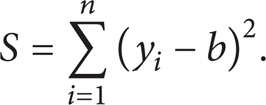
Linearly fit the coordinates as shown in Figure 3, and calculate the standard deviation of the measurement. The fitted line is assumed to have the form y = kx + b. Let

$S={\sum }_{i=\mathrm{1}}^n{d}_i^{\mathrm{2}}={\sum }_{i=\mathrm{1}}^n{\left(\frac{\left|k{x}_i-y_i+b\right|}{\sqrt{k^{\mathrm{2}}+{\mathrm{1}}^{\mathrm{2}}}}\right)}^{\mathrm{2}},$

(9)

where d _i represents the residual, and S is the quadratic sum of residuals. When

$\begin{array}{c}\frac{\partial S}{\partial k}=\mathrm{0},\\ \frac{\partial S}{\partial b}=\mathrm{0},\end{array}$

(10)

the minimum value of S is obtained. If the line is parallel to the x axis, it could be simply expressed as y = b. Thus d _i = y _i – b, and (9) is simplified to

$S={\sum }_{i=\mathrm{1}}^n{\left(y_i-b\right)}^{\mathrm{2}}.$

(11)

The standard deviation of measurement can be obtained by

${\sigma }_m=\sqrt{\frac{S}{n-\mathrm{1}}}.$

(12)

3.2. Elimination and Compensation of Error

(1) Distortion. Due to distortion during imaging, a straight line in object space could appear as a curve in the image plane through projection. There are various distortion models [18–21]. Here a widely used distortion model with 10 parameters is considered [22]. The distortion can be expressed as

$\begin{array}{c}\mathrm{\Delta }x=-x_{\mathrm{0}}-\frac{x^{\prime }}{c}\mathrm{\Delta }c+x^{\prime }{r}^{\mathrm{2}}{K}_{\mathrm{1}}+x^{\prime }{r}^{\mathrm{4}}{K}_{\mathrm{2}}+x^{\prime }{r}^{\mathrm{6}}{K}_{\mathrm{3}}+P_{\mathrm{1}}\left(\mathrm{2}{x}^{\prime \mathrm{2}}+r^{\mathrm{2}}\right)+\mathrm{2}{P}_{\mathrm{2}}{x}^{\prime }{y}^{\prime }+b_{\mathrm{1}}{x}^{\prime }+b_{\mathrm{2}}{y}^{\prime },\\ \mathrm{\Delta }y=-y_{\mathrm{0}}-\frac{y^{\prime }}{c}\mathrm{\Delta }c+y^{\prime }{r}^{\mathrm{2}}{K}_{\mathrm{1}}+y^{\prime }{r}^{\mathrm{4}}{K}_{\mathrm{2}}+y^{\prime }{r}^{\mathrm{6}}{K}_{\mathrm{3}}+\mathrm{2}{P}_{\mathrm{1}}{x}^{\prime }{y}^{\prime }+P_{\mathrm{2}}\left(\mathrm{2}{y}^{\prime \mathrm{2}}+r^{\mathrm{2}}\right),\end{array}$

(13)

where (x₀, y₀) is the principle point, c represents the principle distance, x′ = x – x₀, y′ = y – y₀, and $r=\sqrt{x^{\prime \mathrm{2}}+y^{\prime \mathrm{2}}}$ .

According to the experimental data, when the target image location shift is small enough, the magnitude of the change in the distortion is far smaller than the target locating accuracy. Hence, the influence of distortion has no impact on the comparison of centroid locations. This objective can be achieved through manipulation of the experiment conditions. In this paper, the total shift of target image is about 6 pixels, and the straightness caused by distortion is 1.6 × 10⁻⁵ pixels.

(2) Vibration. Vibration occurs during the image capturing process. Vibration causes shifts in the camera station, thereby shifting the target image locations. Control points were used in order to eliminate the influence of vibration in the experiment. By fixing the control points and target point to the same stable precise platform, the control points do not move. The displacement of a target point is the relative displacement between the target point and the control points. The distribution of target point and control points is as shown in Figure 4.

Figure 4:

Vibration compensation.

Vibrations lead to shifts of control points. The shifts are on the subpixel level as observed in experiments, which is far less than the camera principle distance. For this reason, the shifts for each point in the whole image plane are equal. Compensation for all target points at time i can be obtained by subtracting the control point coordinates at time 0 (x₀′, y₀′) from those at time i (x _i ′, y _i ′).

Consider

$\left(\delta x_i^{\prime },\delta y_i^{\prime }\right)=\left(x_i^{\prime },y_i^{\prime }\right)-\left(x_0^{\prime },y_{\mathrm{0}}^{\prime }\right).$

(14)

The compensated moving target point coordinates are

$\left(x_i,y_i\right)=\left(x_{ai},y_{ai}\right)-\left(\delta x_i^{\prime },\delta y_i^{\prime }\right),$

(15)

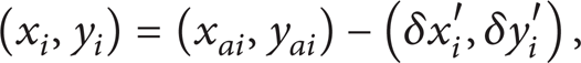
where (x _ai , y _ai ) represents the moving target image point coordinates at time i.

(3) Uncertainty of the Moving Device. Uncertainty of the moving axis in object space is transmitted to the final measurements. It might be necessary to consider this uncertainty if it exceeds a certain range. Assuming that the standard uncertainty in the location of the moving axis is u _c , and the standard uncertainty in the measurement of the target point coordinates is u _m = σ _m , where σ _m is acquired from (12), the standard uncertainty in the target locating method is u. The values of u _c and u are mutually independent, so

$u=\sqrt{u_m^{\mathrm{2}}-u_c^{\mathrm{2}}}.$

(16)

(4) S-Curve Error of Centroiding. The CCD filling factor of the photosensitive material is less than 100%. This results in an S-curve error when centroiding together with the discrete sampling and quantizing. This error fluctuates when the imaged facula is moving in one direction continuously. Thus, it is called the S-curve model [23]. In the experiment in the present study, the target image moves along the x direction of image plane, so this error in the y coordinate does not change, which means that the straightness of the line will not affected by this error. Usually this error can be compensated when centroiding [7, 22].

4. Simulation and Experiment

4.1. Simulation

A simulation was conducted according to the accuracy evaluating method described above. First, pictures of target image were generated. The grayscale level of the inner pixels of target image was set to 200 (of 256 levels) and that of the edge pixels in the target image was set by interpolation according to the illuminated area ratio. The image was smoothed with a Gaussian low-pass filtering function. An appropriate Gaussian noise based on the actual imaging results was then added. Several simulations were conducted to observe the results. The simulated target image was moved in the positive x direction in steps of 0.03 pixels for 200 steps. A target image was generated at each step in a different picture. The target image was then located using different parameters of centroiding. The accuracy of location was acquired from each set of parameter values. Finally, the parameter-accuracy curve and optimal parameter values were obtained. The simulation results are shown in Figure 5 and Table 1.

Table 1:

Simulated error versus parameters α and β.

Error (σ)/pixels versus α
α	i = 0, n = 1	i = 0, n = 2	i = 0, n = 3	i = 0, n = 4	i = 0, n = 5
0.50	0.026175	0.027798	0.024995	0.029100	0.030233
0.75	0.008611	0.010296	0.011212	0.014658	0.017515
1.00	0.003323	0.004663	0.005724	0.007995	0.010601
1.25	0.002090	0.003264	0.004182	0.005854	0.007892
1.50	0.001984	0.003098	0.004087	0.005625	0.007280
1.75	0.002114	0.003227	0.004354	0.005952	0.007437
2.00	0.002302	0.003438	0.004710	0.006429	0.007855
2.50	0.002730	0.003943	0.005496	0.007505	0.008952
3.00	0.003183	0.004492	0.006322	0.008639	0.010188
3.50	0.003648	0.005060	0.007167	0.009794	0.011489
4.00	0.004121	0.005638	0.008022	0.010960	0.012828
Error (σ)/10−3 pixels versus β
β	i = 3, n = 1	i = 4, n = 1	i = 5, n = 1	i = 6, n = 1	i = 7, n = 1
0.1	2.70087	2.66602	2.65650	2.69154	2.66910
1	2.67619	2.65256	2.64703	2.68204	2.66381
2	2.63253	2.63328	2.63369	2.66894	2.65605
3	2.58769	2.60380	2.61620	2.65242	2.64591
4	2.57097	2.57316	2.58985	2.63095	2.63275
5	2.57264	2.56286	2.56254	2.59796	2.61522
6	2.57598	2.56466	2.55091	2.56451	2.58725
7	2.58076	2.56713	2.55092	2.55493	2.56290
8	2.58713	2.57118	2.55111	2.56179	2.55759
9	2.59605	2.57529	2.55309	2.56783	2.56049
10	2.60361	2.57813	2.55453	2.57192	2.56250

Figure 5:

Simulated error versus parameters α and β.

In Figure 5, n is the standard deviation of the noise added in simulation, and μ is the mean. The unit is one increment of grayscale intensity. As can be seen in Figure 5 (a), for any case of n = 1 to 5 (based on experience, the actual noise of the imaging process will not ordinarily exceed this range), there is a minimum locating error which is close to α = 1.5. Figure 5 (b) shows that the accuracy versus β curve has a minimum value as well for each noise level. Some of the data are shown in Table 1.

As seen in Table 1, α contributes much more to accuracy improvement than β. When α = 1.5, it resulted in 30% and 10% accuracy improvement compared to centroiding and squared centroiding, respectively. Additionally, β contributed about 4% to the accuracy for each noise value μ. The best β value is slightly larger than the expected value of noise. That is because the noise does not have an effect if it is negative in background pixels.

4.2. Experiment

A Nikon D2Xs camera, whose interior parameters have been calibrated, was used in the experiment. The pixel size of the camera was 6 μm × 6 μm, and the resolution was 4288 × 2848 pixels. A Hexagon Mistral 775 coordinate measuring machine (CMM) was used for high-precision movement of the target point. Accuracy of movement depends on the grating scale accuracy, which was 0.1 μm. Retro-reflective target points were used for imaging. The diameter of the targets was 6 mm. The target image facula diameter was about 10 pixels. The experiment was implemented under favorable environmental conditions.

A flow diagram of the experiment is shown in Figure 6.

Figure 6:

Flow diagram of the experiment.

Figure 7 shows the experimental scenario. The target in the middle is the measuring target point. There is a column of vibration compensation control points fixed on the CMM platform on both sides of the target. To facilitate comparison, all points are located in a plane, the optical axis of the camera is perpendicular to this plane, and the initial position of the target image center is imaged near the principle point. The camera is fixed on an optical table and set for automatic image capture. The target object moves 200 steps in steps of 30 μm in the positive x direction, and 201 pictures are taken as one group of data. For reliable results, 10 groups of data were collected at different times.

Figure 7:

Experimental platform and RRT distribution.

The target image is located with variable grayscale-weighted centroiding for all 10 groups of data. The first group of data is taken as an example to analyze the influence of lens distortion. The point moves from (2160.4423, 1248.7070) to (2166.4188, 1248.7090) in the image plane. The shift in the y direction is 0.002 pixels. Equation (13) and the camera parameters are used to calculate the distortion. A distortion value sequence {(Δx₀, Δy₀), (Δx₁, Δy₁), …, (Δx _i , Δy _i ), (Δx₂₀₀, Δy₂₀₀)} which has a straightness of about 1.6 × 10⁻⁵ pixels and a standard deviation about 4 × 10⁻⁶ pixels is obtained. This distortion is small enough to be ignored. Equations (14) and (15) and the control points coordinates are used to compensate for vibration errors. Since the target image moves in the x direction, the S-curve error in y direction does not change; therefore, this error causes no deviation. The standard deviation (σ _m ) of the residuals is obtained by linear fitting the coordinate sequence of each group of data. For the seeking of optimal values of α and β, there must be a α-σ _m curve and a β-σ _m curve for each picture group. Equation (16) is used to decompose the influence of target object locating uncertainty. Finally, the accuracy of the target image locating, the parameter-accuracy curve, and the optimal parameter value are obtained. The average of the experiment results is shown in Figure 8 and Table 2. Selected data are listed in Table 2.

Table 2:

Measured error versus parameters α and β.

Error (σ) versus α				Error (σ) versus β
α	Error (σ)	α	Error (σ)	β	Error (σ)	β	Error (σ)
0.50	0.019177	2.00	0.006589	0	0.005853	6	0.005872
0.75	0.010303	2.50	0.007486	1	0.005847	7	0.005886
1.00	0.006875	3.00	0.008423	2	0.005845	8	0.005901
1.25	0.005913	3.50	0.009372	3	0.005847	9	0.005918
1.50	0.005894	4.00	0.010321	4	0.005852	10	0.005936
1.75	0.006189	4.50	0.011267	5	0.005861	11	0.005953

Figure 8:

Measured error versus parameters α and β.

According to the experimental data, there are minimum errors in both the α-σ _m and β-σ _m curves. The minimum locating error is close to the position of α = 1.5, which is the same as in the simulation result. When α is 1.5, the locating error σ is 1/170 pixels, and β has little effect on accuracy.

An additional experiment was conducted to determine the relationship between optimal α or β values and the target image location. Figure 9 shows how 8 groups of data were acquired with different target locations and moving directions. The results are shown in Figure 10. The data show that the optimal α value is always between 1.25 and 1.75 with an average of 1.505. This α value results in accuracy improvements of 18.4% and 10.2% compared with the centroid and squared centroid methods, respectively. The optimal β value is between 0 and 6. Still, β contributes little to accuracy improvement.

Figure 9:

Target location and moving direction.

Figure 10:

Optimal α and β values versus target location.

5. Conclusion

This paper derives a general algorithm for grayscale-weighted centroiding method. The general algorithm sets weight as a function of grayscale intensity and two undetermined parameters α and β where α is the weighted index, and β is the grayscale shift. This paper analyzed and demonstrated the existence of minimum error in the domain of variability of α and β, and then designed an accuracy evaluating method to obtain the accuracy of a centroid with specific α and β values. Finally the accuracy-α and accuracy-β curves can be obtained by discrete sampling of α and β values as well as the optimal centroiding location. Simulations and experiments were conducted to confirm the accuracy improvement of this method. Results show that the optimal value of α improves locating accuracy more effectively than β. When α = 1.5, both simulation and experimental results exhibit an improvement of accuracy by 10% compared to squared centroiding, while β contributes about 1% to accuracy improvement. Locating accuracy shows a distinct improvement overall. This means that more accurate target location coordinates can be provided to 3D reconstruction and bundle adjustment. It paves the way to improve accuracy of photogrammetry.