Resonance-Based Nonlinear Demodulation Analysis Method of Rolling Bearing Fault

Abstract

Numerous mechanical nonstationary fault signals are a mixture of sustained oscillations and nonoscillatory transients, which are difficult to efficiently analyze using linear methods. We propose a nonlinear demodulation analysis method based on resonance and apply it to the fault diagnosis of rolling bearings. Unlike conventional demodulation methods that use frequency-based analysis and filtering techniques, our nonlinear demodulation analysis method is a decomposition demodulation of the signals according to different resonance based on Q-factors. When a local rolling bearing fault such as pitting is present, the fault vibration signals consist of the regular vibration signals and noise (a high resonance component containing multiple simultaneous sustained oscillations) and a transient impulse signal (a low resonance component being a signal containing nonoscillatory transients of faults). The regular vibration signal is a narrowband signal that has a high Q-factor, and the transient impulse signal is a wideband signal that has a low Q-factor. Using our resonance-based nonlinear demodulation analysis method, we decompose the signal into high resonance, low resonance, and residual components. Then, we perform a demodulation analysis on the low resonance component that includes the fault information. We have verified the feasibility and validity of the algorithm by analyzing the results of experimental and engineering signals.

1. Introduction

The rolling bearing is one of the most widely used general mechanical components in rotating machines. Its running state directly affects the performance of the whole machine. Detecting and diagnosing its faults can prolong service life and reduce production costs. Therefore, it is important to monitor the bearing's condition to ensure operational safety, prevent serious accidents, and reduce production costs [1].

The local fault vibration signal of a rolling bearing is a typical nonstationary signal. Compared with a stationary signal, the distribution parameters and regularities of the rolling bearing fault vibration signal are time dependent. Moreover, massive noise can be inevitably introduced into its vibration signal during the generation and transmission process, because of complex operational conditions and harsh environments. This is a major inconvenience to the analysis, handling, and use of the signals. When the inner ring, outer ring, or the rolling element of the rolling bearing is damaged, a periodic mechanical impact occurs in the contact between the surface of the fault and the surfaces of other elements within the cyclic rotation of the bearing. This arouses the natural frequency of the rolling bearing, and a periodic transient impulse signal occurs in its vibration signal, forming a modulation phenomenon. Consequently, the key to the fault diagnosis of a rolling bearing is to determine the algorithm for extracting the periodic impulse component and a demodulation analysis of the nonstationary multicomponent modulation signal with massive noise. A nonstationary modulation signal always exists in practical projects, so it is important to investigate this kind of signal.

Traditional envelope demodulation methods can be classified into Hilbert transform demodulation analysis or generalized detection-filtering demodulation analysis [2–4]. However, both have limitations: two time domain adding signals that have no fault information are demodulated by subtracting their frequencies [5]. Thus, the demodulation signal should be preprocessed. Currently, the signals are preprocessed using methods based on signal frequency or scale, such as the Fourier and wavelet transforms [6–10] or empirical mode decomposition (EMD) [11–13]. It is hard to use wavelet transforms for complicated signals because of the singleness of their basic decomposition functions, and the wavelet function is hard to determine. In addition, when the frequencies of the interference element of the signal and the valid impacting component overlap, the latter cannot be demodulated and analyzed using wavelet decomposition demodulation analysis methods. As an adaptive signal processing method, EMD has an effect on the feature extraction of a fault signal. However, the EMD method is essentially an orthogonal band-pass filter bank. When a sustained periodic oscillation signal and a transient impulse signal overlap on the bands, the periodic vibration jamming signal and the transient impulse component cannot be efficiently separated. There are also theoretical problems in the EMD method such as overenveloping, underenveloping, and mode mixing, and thus further studies are necessary.

Selesnick lately proposed the resonance-based sparse signal decomposition method [14], which is different from the traditional signal decomposition approach based on the frequency or scale. In this approach, according to the difference between the quality factors (defined as the ratio of central frequency and the frequency bandwidth and denoted as Q-factor) of transient impulse signal and sustained oscillation periodic signal, a complex signal is decomposed into the high resonance component consisting of sustained oscillation part and the low resonance component consisting of the transient impulse part. The transient impulse signal is wideband signal, possessing low Q-factor. However, the sustained vibrating periodic signal is narrowband signal, possessing high Q-factor. Consequently, based on the difference between Q-factors, transient impulse signal and sustained vibrating periodic signal could be effectively separated. In the resonance-based sparse signal decomposition method, two Q-factors, one with high value and the other with low value, are selected according to the signal to be analyzed, before the establishment of the sparse representation forms of high resonance component and low resonance component using tunable Q-factors wavelet transform. Then, the sparse decomposition target function is established with the morphological analysis method. In the end, the split augmented Lagrangian shrinkage algorithm is utilized to optimize the solution to get the high and low resonance components of the signal.

In this study, we introduce the resonance-based sparse signal decomposition method to the fault diagnosis of rolling bearings. We propose a technique for fault nonlinear demodulation analysis of rolling bearings based on resonance. Our approach uses a combination of a high resonance component (sustained oscillation component) and a low resonance component (transient impulse component) to represent the nonstationary multicomponent modulation signal of the rolling bearing fault. The transient impulse component is a wideband signal, which possesses a low Q-factor, while the sustained oscillation periodic component is a narrowband signal with a high Q-factor. Therefore, based on the difference between Q-factors, we construct compound Q-factor bases (high and low Q-factor bases). The high Q-factor base is used to match the high resonance component (the random vibration and strong noise of the rolling bearing itself). The low Q-factor base is used to match the low resonance component (fault impulse component). Finally, we analyze the fault impulse component for demodulation. Then, we conduct the fault diagnosis based on the demodulation spectrum. The results of simulation and application analyses show that our method can make a quick and accurate demodulation analysis, extract the impact features, and overcome the limitations of demodulation analysis based on frequencies. Thus, we provide a new method for the study and analysis of nonstationary multicomponent modulation signals of rolling bearing faults.

The paper is organized as follows. Section 2 presents the sparse decomposition based on the compound Q-factor bases and the steps of the nonlinear demodulation analysis method. Section 3 describes the simulated signal analysis results. Section 4 presents an analysis of the experimental signal. We further validate the algorithm using an analysis of an engineering example in Section 5. Finally, Section 6 concludes the paper and includes some remarks regarding future work.

2. Signal Decomposition Based on Compound Q-Factor Bases

2.1. Annotation of Resonance of Signal

It has been discussed in [14] that a complex nonstationary signal is a mixture of a sustained oscillation component (high resonance component) and a nonoscillation transient component (low resonance component). A resonance-based sparse decomposition algorithm has been proposed and applied to the processing of complex voice signals, with satisfactory results. The simulation signal in Figure 1 can be used to effectively explain the concept of signal resonance. Signal 1 (f = 3 Hz) and Signal 3 (f = 10 Hz) are defined as low resonance signals (Q-factor = 1), because neither has sustained oscillations. Signal 2 (f = 3 Hz) and Signal 4 (f = 10 Hz) are defined as high resonance signals (Q-factor = 6), because they do have sustained oscillations. As a result, both the high and low resonance signals can concurrently contain low-frequency and high-frequency signals. The high resonance signal can be sparsely represented by a basis function with a high Q-factor, while the low resonance signal can be represented by a basis function with a low Q-factor.

Figure 1:

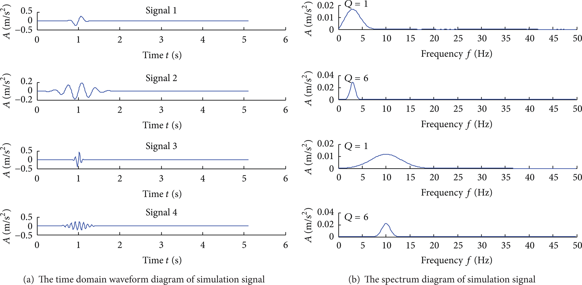
High resonance signal and low resonance signal.

2.2. Construction of Compound Q-Factor Bases

The tunable Q-factor wavelet transform is a complete discrete wavelet transform. The value of the Q-factor of a wavelet function can be arbitrarily adjusted and can be adaptively designed and selected according to the oscillations of the analyzed signal [15–17]. This is what is needed to construct the Q-factor base. Therefore, we propose a basis function library for obtaining high and low Q-factor transforms that exploit tunable Q-factor wavelet transforms. Then, the high and low Q-factor bases are chosen and used for the sparse representation of the high and low resonance components of the fault signal of the rolling bearing. We construct the corresponding Q-factor bases using band-pass filter banks based on the tunable Q-factor wavelet transform. The two groups of band-pass filter banks are shown in Figure 2.

Figure 2:

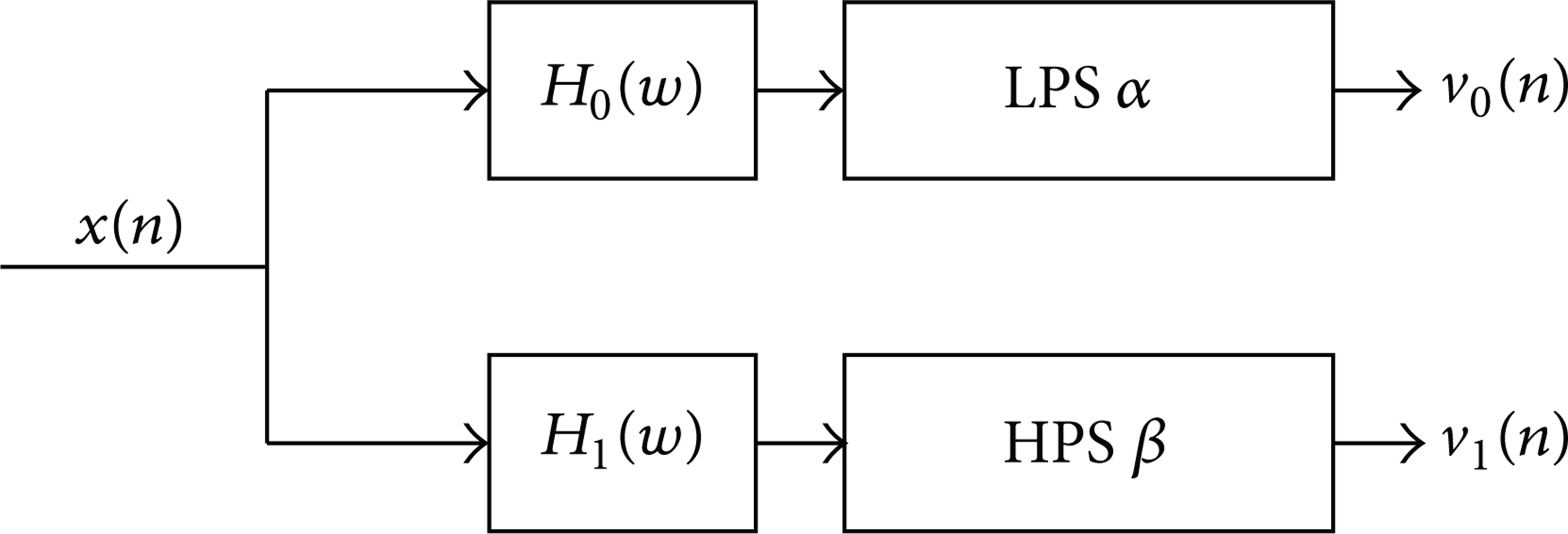
Flow chart of tunable Q-factor wavelet transform.

In Figure 2, β is the high pass scaling factor, and α is the low pass scaling factor such that

$\beta =\frac{\mathrm{2}}{Q+\mathrm{1}},\hspace{1em}\hspace{1em}\alpha =\mathrm{1}-\frac{\beta }{r}.$

(1)

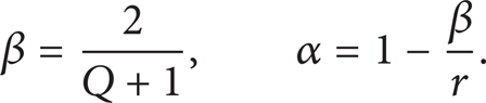
And the scaling factors, α and β, satisfy

$\mathrm{0}<\alpha <\mathrm{1},\hspace{1em}\hspace{1em}\mathrm{0}<\beta <\mathrm{1},$

(2)

where r is the redundancy, x(n) is the signal for analysis, v₀(n) is the extracted low resonance component, and v₁(n) is the extracted high resonance component.

When the scaling factors α and β are determined, we calculate the values of the Q-factor and r. Figure 3 is a simple example of the high and low Q-factor bases produced by adjusting the scaling factors α and β.

Figure 3:

The diagram of high Q-factor and low Q-factor.

From Figure 3, it can be seen that the extent of the sustained oscillations of the high and low Q-factor bases is different. Hence, the changing Q-factor wavelet transform can be used to construct the corresponding high and low Q-factor bases and, therefore, extract the high and low resonance components (fault impact components) of the nonstationary signal of the rolling bearing fault.

2.3. Sparse Representation of High Resonance Component and Low Resonance Component with Compound Q-Factor Bases

The sparse signal decomposition method based on compound Q-factor bases uses morphological component analysis to perform a nonlinear separation of the components in the signal according to the oscillation feature [18–20]. Then, we establish the best sparse representation forms of the high and low resonance components.

Assume that the observed signal, x, can be represented by the sum of two component signals x₁ and x₂,

$x=x_{\mathrm{1}}+x_{\mathrm{2}}\hspace{1em}x,\hspace{0.17em}{x}_{\mathrm{1}},\hspace{0.17em}{x}_{\mathrm{2}}∊R^N.$

(3)

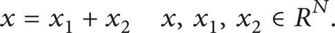
The purpose of morphological component analysis is to estimate the source signals, x₁ and x₂, from the observed signal, x. We can assume that x₁ and x₂ can be represented by the basis function libraries (or frames) S₁ and S₂ (where S₁ and S₂ have low correlation). x₁ and x₂ in this study denote the high and low resonance components of the signal, respectively. S₁, S₂ denote the high and low Q-factor bases obtained from the filter banks of the changing Q-factor wavelet transform. A target function of the morphological component analysis can be expressed as

$J\left(w_{\mathrm{1}},w_{\mathrm{2}}\right)={\parallel x-S_{\mathrm{1}}{W}_{\mathrm{1}}-S_{\mathrm{2}}{W}_{\mathrm{2}}\parallel }_{\mathrm{2}}^{\mathrm{2}}+{\lambda }_{\mathrm{1}}{\parallel W_{\mathrm{1}}\parallel }_{\mathrm{1}}+{\lambda }_{\mathrm{2}}{\parallel W_{\mathrm{2}}\parallel }_{\mathrm{1}},$

(4)

where W₁ and W₂ denote the transformation coefficients of the signals x₁ and x₂ under the frames S₁ and S₂, respectively, and λ₁ and λ₂ denote the regularization parameters. The choices of λ₁ and λ₂ have an impact on the energy distribution of the decomposed, high resonance component and low resonance component. For a given λ₂, increasing λ₁ decreases the energy of the component corresponding to λ₁. If λ₁ and λ₂ increase at the same time, the residual signal would have a higher energy.

In (4), the l₁ norm is nondifferentiable and has a considerable number of parameters, so it is difficult to solve [10]. The sparse signal decomposition method based on compound Q-factor bases uses the split augmented Lagrangian searching algorithm. It minimizes the target function, J, by iteratively updating the transform coefficients W₁ and W₂. Eventually, it effectively separates the high resonance component and low resonance component and extracts the transient impulse component.

Assume that the transform coefficients of the high and low Q-factors corresponding to the minimized target function J are W₁^* and W₂^*. Then, the estimated values of the high and low resonance components (solved by matching) are represented by

$\widehat{x_{\mathrm{1}}}=S_{\mathrm{1}}{W}_{\mathrm{1}}^{*},\hspace{1em}\hspace{1em}\widehat{x_{\mathrm{2}}}=S_{\mathrm{2}}{W}_{\mathrm{2}}^{*}.$

(5)

2.4. Nonlinear Demodulation Analysis Steps of Fault Diagnosis of Rolling Bearing with Compound Q-Factor Bases

The high and low Q-factors, Q₁ and Q₂ (normally Q₁ = 3 and Q₂ = 1), the transform redundancy of the high and low Q-factors, r₁ and r₂ (normally r₁ = r₂ = 3), and the transform decomposition level number of the high and low Q-factors, J₁ and J₂, are selected according to the fault signal of the rolling bearing, x. In this study, these values are chosen to be Q₁ = 3, Q₂ = 1, r₁ = r₂ = 3, J₁ = 22, and J₂ = 10.

Using the parameters in Step (1), we obtain the basis function libraries S₁ and S₂ of the high and low Q-factor wavelet transfers. The basis function libraries are used to transform the fault signal, x, of the rolling bearing. Thus, the initial transform coefficients W₁ and W₂ are obtained.

The regularization parameters, λ₁ and λ₂, are determined (in this study, λ₁ = λ₂ = 0.5). Then, we establish the target function J (4). Next, the split augmented Lagrangian algorithm is used to estimate the optimal transform coefficients of W₁^* and W₂^*.

Equation (5) is used to reconstruct the signal with the coefficients W₁^* and W₂^*, to obtain the high and low resonance components of the signal using the compound Q-factor base.

We conduct a demodulation analysis on the low resonance component, which is then used to diagnose the fault of the rolling bearing.

3. Simulation Signal Analysis

To test and verify the validity and superiority of the nonlinear demodulation analysis method based on resonance, we have applied it to fault characteristic extraction in the simulation of a rolling bearing.

We will now describe the basic idea behind simulating a bearing fault in a gearbox. We use a periodic impulse signal to simulate the vibration characteristic frequency of a single fault of the bearing. We superimpose an exponential attenuating high-frequency harmonic signal on it to simulate the natural frequency of the gearbox system. A low-frequency harmonic signal is added to simulate the low-frequency interference from imbalances, misalignments, and mechanical looseness. We add random noise to simulate environmental interference. In this study, the high-frequency harmonic signal of the exponential attenuation is

$x=e^{-\mathrm{3000}t}\cos \left(\mathrm{2}\pi ·\mathrm{720}·t\right).$

(6)

The frequency of the periodic pulse impulse signal that models the vibration characteristic frequency of the single fault of the bearing is f _c = 90 Hz. It is used to modulate the high-frequency harmonic signal mentioned above. The sampling frequency of the signal is 8192 Hz, with 4096 sampling points and 0.5 seconds duration. The time domain waveform and the spectrogram of the obtained periodic impulse signal are shown in Figures 4 (a) and 4 (b). Figure 4 (c) is its demodulation spectrum. From the figures, we can see that the demodulation spectrum is mainly made up of f _c and its harmonic component.

Figure 4:

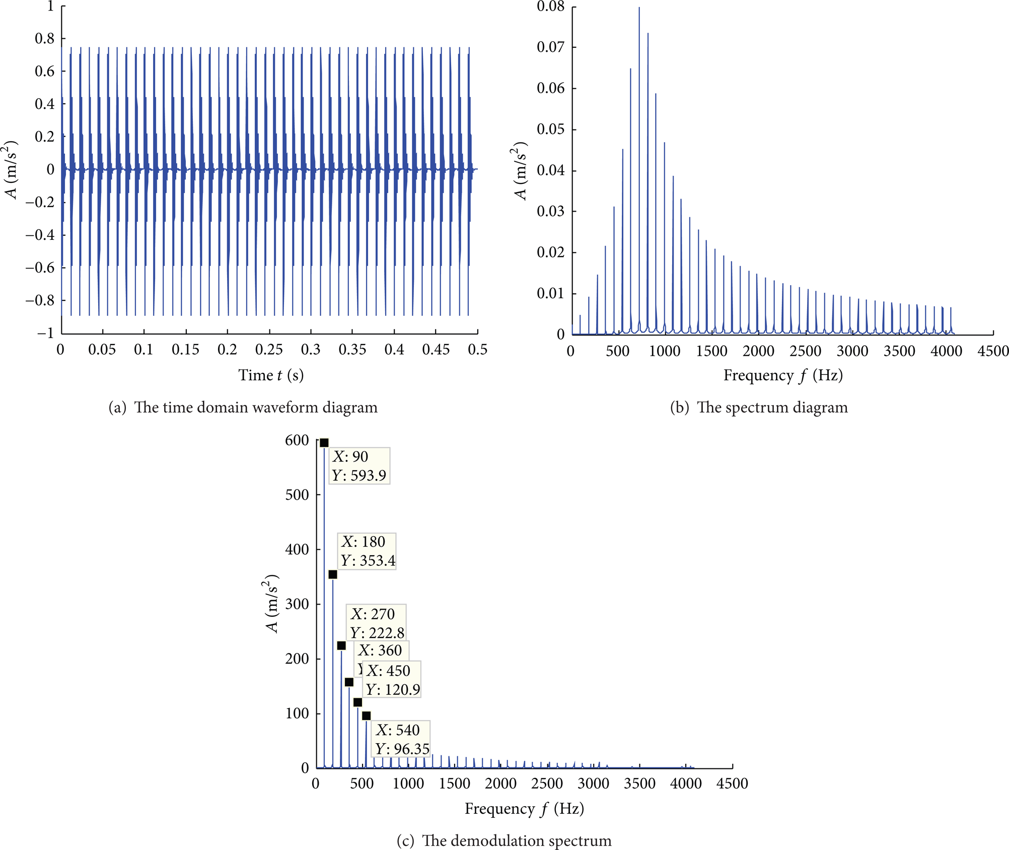
The time domain waveform, spectrum diagram, and demodulation spectrum of periodic impact signal.

The periodic impulse signal shown in Figure 4 (a) is added to sinusoidal low-frequency interfering signals that have frequencies of f₁ = 650 Hz and f₂ = 800 Hz and amplitudes of 1 (at this time, the spectrum of the sinusoidal signal overlaps with the periodic impulse spectrum). We continuously add a Gaussian noise (SNR = – 5). The time domain waveform of the obtained simulated signal is shown in Figure 5 (a). It can also be seen in this figure that the impulse signal is hidden.

Figure 5:

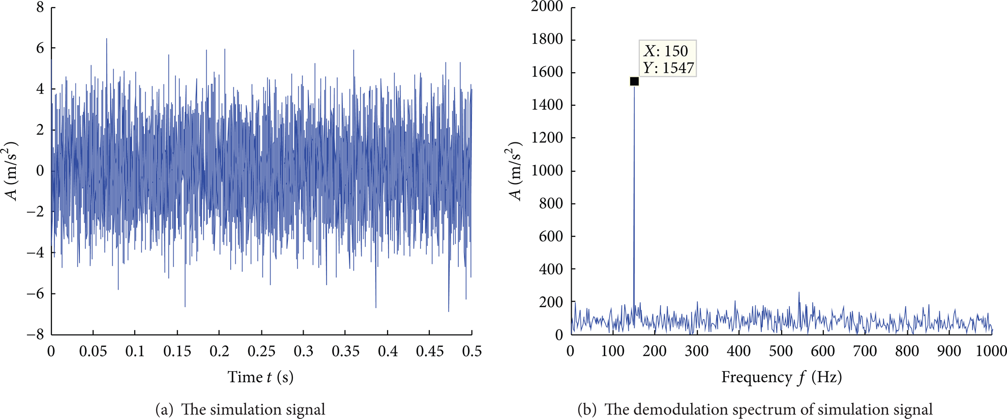
The time domain waveform diagram and demodulation spectrum of simulation signal.

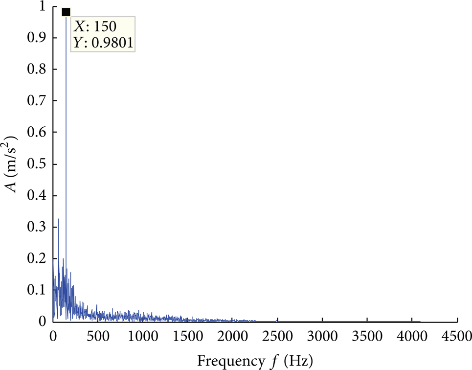
We use the Hilbert envelope demodulation to effectively analyze the signal. The obtained demodulation spectrum is shown in Figure 5 (b). The base frequency (150 Hz) and its harmonic component can be seen in the demodulation spectrum of Figure 6; that is, we can only obtain the frequency difference of the low-frequency interference component and not the frequency of the impulse signal. Therefore, for an accurate analysis, the simulated signal needs to be preprocessed before the demodulation analysis.

Figure 6:

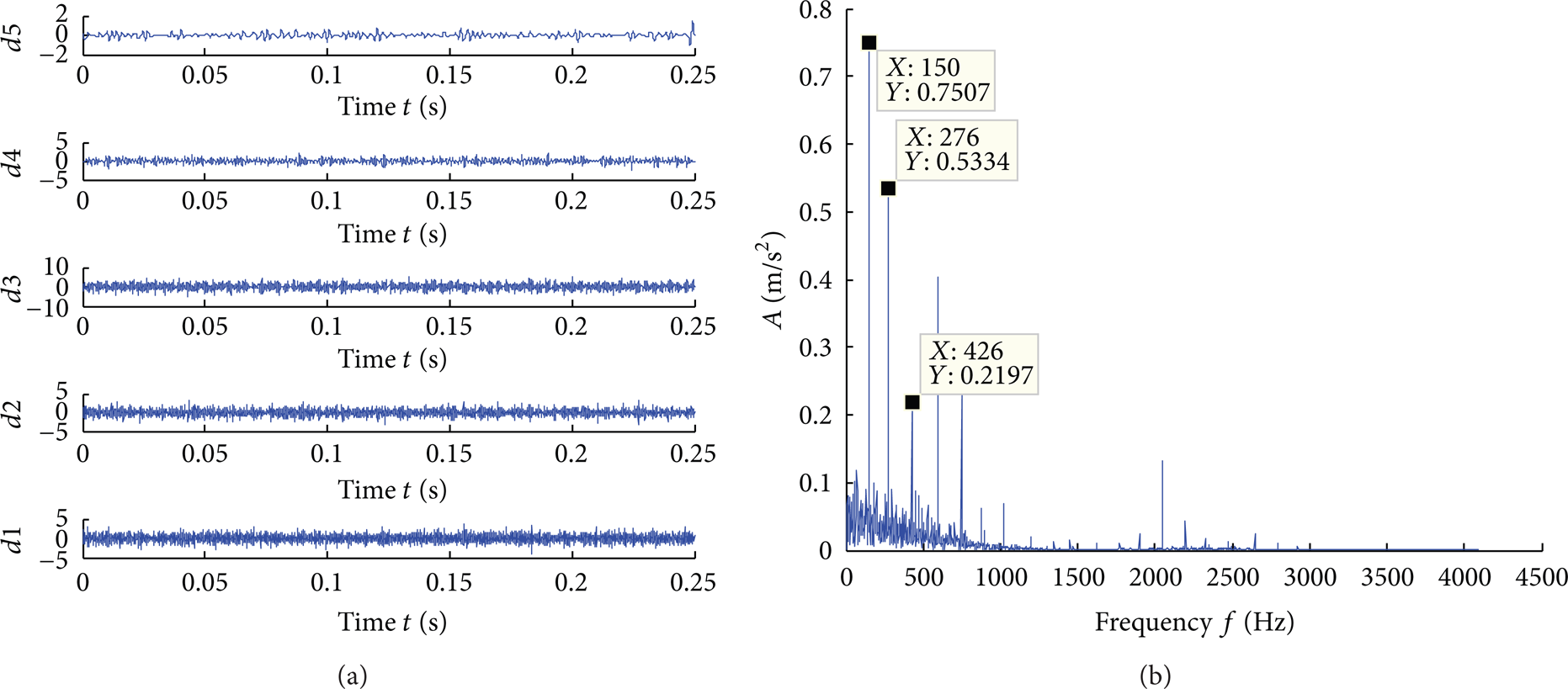
(a) The wavelet decomposition of signal. (b) The demodulation spectrum of d3.

The simulated signal is decomposed into five levels using wavelet decomposition. The decomposed signals are shown in Figure 6 (a). We chose d3 for the demodulation analysis. The result is shown in Figure 6 (b).

We can only see the frequency of f = 150 Hz in the demodulation spectrum of Figure 6 (b); so we have not overcome the problems of traditional envelope demodulation by preprocessing the wavelet decomposition.

Hence, we still need to use the EMD method, because it has the ability to adaptively decompose the composite signal. Figures 7 (a) and 7 (b) show the obtained signal pattern components.

Figure 7:

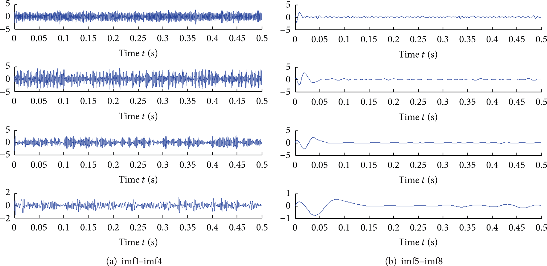
Model component diagram of signal decomposition.

It can be seen from Figure 7 that the EMD method decomposes the simulated signal into 8 pattern components, imf1–imf8. We then calculated the correlation coefficients of the signal and the compound signal. The results show that the correlation coefficient between imf2 and the simulation signal is the largest, being 0.9192. Hence, we used imf2 for demodulation analysis. The obtained demodulation spectrum is shown in Figure 8.

Figure 8:

The demodulation spectrum of imf2.

The demodulation spectrum of imf2 in Figure 8 only shows a frequency of f = 150 Hz. This means that the EMD decomposition preprocessing was not able to overcome the problems of traditional envelope demodulation. Consequently, we used the signal decomposition method based on compound Q-factor bases to decompose the signal. We obtained the results shown in Figures 9 (a), 9 (b), and 9 (c). Figure 9 (a) shows the periodic elements with frequencies of f₁ and f₂. Figure 9 (b) shows that the impulse component of the low resonance component is obvious and that the time interval between impulses coincides with the impulse interval of Figure 4 (a). The residual signal in Figure 9 (c) is the difference between the primary signal and the high and low resonance components, which is the signal reconstruction error. It is clear that the residual signal possesses a rather low energy, indicating that the sparse decomposition method based on compound Q-factors creates a better reconstruction. The purpose of our algorithm is to extract the low resonance impulse component, so we do not show the residual component in the rest of this paper.

Figure 9:

(a) The high resonance component. (b) The low resonance component. (c) The residual component. (d) The demodulation spectrum of low resonance component.

The envelope spectrum shown in Figure 9 (d) was obtained after conducting the demodulation analysis of the low resonance component in Figure 9 (b). The spectral peak of the figure mainly consists of f _c and its harmonic component. By comparing this with Figure 4 (c), we can see that the envelope demodulation spectrum based on sparse signal resonance decomposition is successful at extracting the modulation information of the impulse signal. This validates the effectiveness of our method. Further comparisons with the wavelet decomposition demodulation spectrum shown in Figure 6 (b) and the EMD decomposition demodulation spectrum shown in Figure 8 demonstrate the advantages of our method.

4. Analysis of Experimental Signal

4.1. Analysis on the Experimental Signal of the Single Fault of the Rolling Bearing

The experimental data is collected from the Internet [21]. The experimental system is shown in Figure 10. It consisted of a motor with 2 horsepower (left), a torque transducer/encoder (central), a dynamometer (right), and control electronics (not shown). The test bearing supported the motor shaft. The deep groove ball bearing produced by the SKF company was used as the test bearing (model 6205-2RS JEM SKF). The bearing inner ring was processed with an electric spark to produce a single fault. The diameter of the fault was 7 mils (1 mil = 0.001 inches), while the motor speed was n = 1797 r/min. The vibration data was collected by an accelerometer sensor with its magnetic base attached to the case. The vibration signal was collected by a 16-channel DAT recorder and postprocessed using Matlab 8.1. The speed of data collection was 12,000 samples per second (sampling frequency f _s = 12,000 Hz). The characteristic fault frequency of the bearing inner ring was f = 162.2 Hz.

Figure 10:

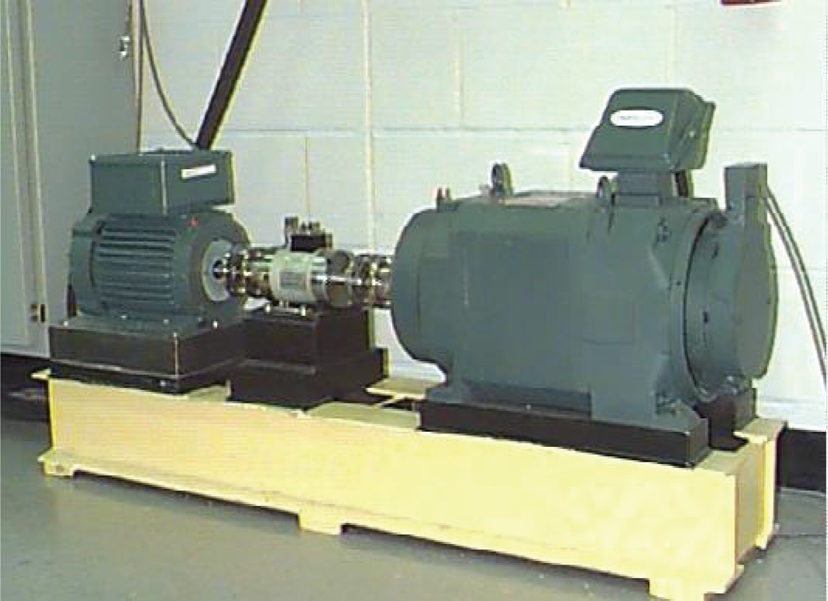
The experiment system.

The experimental data of the fault of the measured bearing inner ring is chosen to be analyzed. The time domain and spectrum graphs are shown in Figure 11.

Figure 11:

The original signal time domain waveform diagram and spectrum diagram.

We performed a sparse decomposition of the signal shown in Figure 11 using compound Q-factor bases. The obtained low resonance component is shown in Figure 12. We can see that the low resonance component has a clear impulse component. We used envelope demodulation on the impulse component, and the resulting spectrum is shown in Figure 13. We can infer from Figure 13 that the frequency is 161.1 Hz (inner ring fault characteristic frequency). This is its multiplication frequency component. Consequently, we have diagnosed the inner ring fault in the rolling bearing, as required. This validates the effectiveness of our nonlinear demodulation method based on resonance.

Figure 12:

The low resonance component.

Figure 13:

The demodulation spectrum of low resonance component.

4.2. Analysis of Compound Fault Experiment Signal of Rolling Bearing

The experimental system consisted of a gearbox test bed, a HG3528A data acquisition instrument, and a laptop. The data acquisition instrument uploaded the collected data to the computer for processing and analysis. The test bed of the gearbox is shown in Figure 14. The driven shaft of the gear box was supported by two 6307 bearings; one was functioning normally and the other was pitted. The motor revolved constantly at a speed of n = 1496 r/min. The major diameter of the bearing was D = 80 mm, the minor diameter was d = 35 mm, the number of rolling elements was Z = 8, and the contact angle was a = 0. The simulated compound fault included the pitting fault of the outer and inner rings of the bearing. The pitting fault was a 1 mm dimple, at a depth of 0.2 mm. We substituted the above parameters into the corresponding formulas and determined that the fault characteristic frequency of the bearings outer ring was 76.7 Hz, of the inner ring was 122.7 Hz, and of the rolling element was 51.1 Hz. There were 8192 sampling points and the sampling frequency was 15360 Hz.

Figure 14:

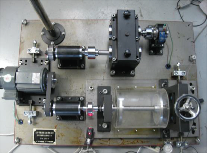
The experiment system of gearbox.

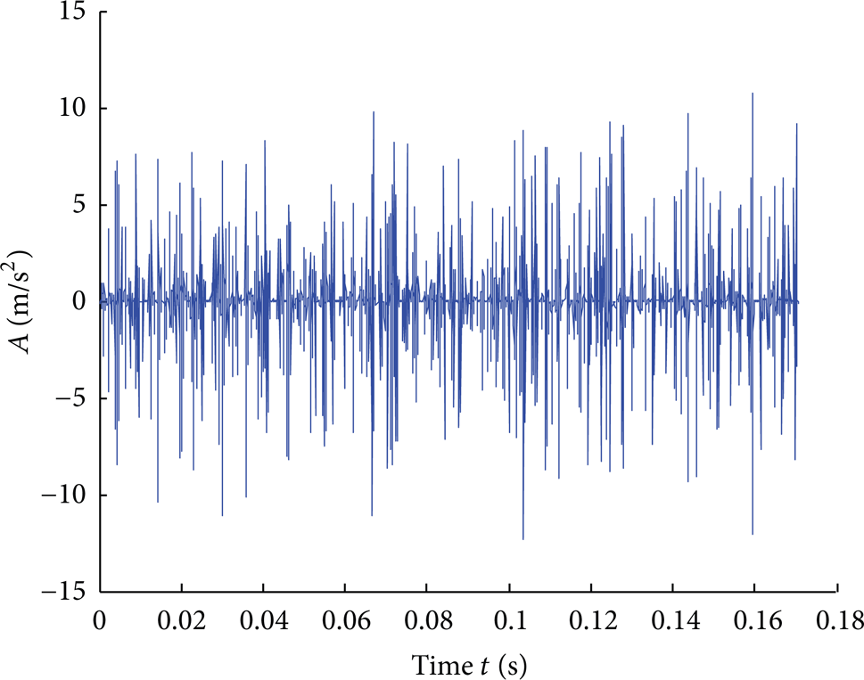
We chose to analyze the experimental data of the compound pitting fault. The time domain and the spectrum graphs are shown in Figure 15. The impulse component was not obvious, so the fault characteristic needed to be further extracted.

Figure 15:

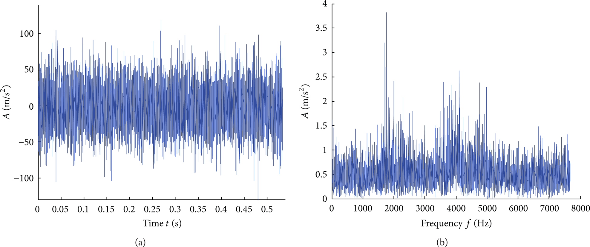
The original signal time domain waveform diagram and spectrum diagram.

We used a sparse decomposition based on compound Q-factor bases to extract the signal shown in Figure 15. The obtained low resonance component is shown in Figure 16. It is clear that the low resonance component has a clear impulse component. The spectrum derived after envelope demodulation is shown in Figure 17. In this figure, we can see the frequency of 76.88 Hz (the outer ring fault characteristic frequency) and its frequency multiplication component and the frequency of 121.9 Hz (the inner ring fault characteristic frequency) and its frequency multiplication component. Thus, we can diagnose the bearing's inner and outer ring fault. These results further prove the effectiveness of the sparse decomposition demodulation analysis method based on compound Q-factor bases.

Figure 16:

The low resonance component.

Figure 17:

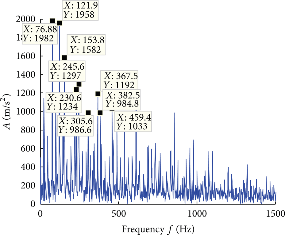
The demodulation spectrum of low resonance component.

5. Analysis of Bearing Fault Engineering Signal

To further verify the effectiveness and superiority of the compound Q-factor bases, we analyzed some engineering data.

There was a teeth collision incident in the gearbox of the wire rod 27th finishing mill in a steel plant at 18:32 on September 22, 2007. The fault was in the 12th bearing of Shaft II. The whole bearing was badly damaged, resulting in a 6-hour suspension. The transmission chains of this wire rod finishing mill gearbox are shown in Figure 18. The detected signal of the system at this position shows that the peak alarm rang before the incident but did not continue, and so the incident occurred. We gathered data obtained two hours before the incident, that is, at 16:00. The number of sampling points was 2048, and the sampling frequency was 12,000 Hz. The primary signal wave is shown in Figure 19. No obvious impulse characteristic can be seen. We used the compound Q-factor bases for the sparse decomposition of the signal. We obtained the low resonance component, as shown in Figure 20. The periodic impulse signal component can be seen. Its demodulation spectrum is shown in Figure 21. The fault characteristic frequency of 193.4 Hz and its frequency multiplication are clear, which almost coincides with the theoretical outer fault characteristic frequency of the rolling bearing (191.18 Hz). The relative error is only 1.16%.

Figure 18:

The gearbox transmission chain chart.

Figure 19:

The original signal time domain waveform diagram.

Figure 20:

The low resonance component.

Figure 21:

The demodulation spectrum of low resonance component.

6. Analysis of Normal Bearing Signal

In the paper, it is shown that the method can effectively detect faults that some other methods cannot detect. In order to show how the method works when no faults are present, we analyze the normal bearing data. The time domain graph is shown in Figure 22.

Figure 22:

The normal bearing signal time domain waveform diagram.

The proposed method is performed on the signal shown in Figure 22. The obtained resonance component is shown in Figure 23.

Figure 23:

(a) The high resonance component. (b) The low resonance component.

It can be seen that the high resonance component is the same as the normal bearing signal. Meanwhile the low resonance component is zero. So we can draw the conclusion that there are no faults in the bearing and demonstrate the behavior of the proposed method on data where there are no faults and show that the method does not produce false positives.

7. Conclusion

Unlike traditional signal decomposition methods that use frequency division, our nonlinear demodulation method is based on resonance. It uses the difference in the Q-factors of the transient impulse and background noise to decompose the signal into a high resonance component with background noise and a low resonance component with a transient impulse. Thus, this method effectively achieves the separation of background noise and transient impulse.

Conventional demodulation analysis methods based on frequency would treat the interfering signal and exclude the fault signal as the defect was solved using the demodulation frequency. To overcome this, we proposed a nonlinear demodulation analysis method based on resonance to analyze the nonstationary multicomponent modulation signal of the rolling bearing. When the periodic interfering signal component is removed, the fault of the rolling bearing can be effectively diagnosed. In future studies, we shall consider the effect of fault diagnosis on other rotating machinery.