A Location Prediction Algorithm for Mobile Communications Using Directional Antennas

Abstract

A directional communication scheme, TRAC, is proposed in this paper to deal with issues in mobile directional communications. Directional communication can bring benefits in terms of spatial reuse, power consumption, and security. Using direction antennas implies that the transmitters must know the direction or location of the receiver. It is necessary to predict the receiver's location to keep the transmitter's antenna pointing in the right direction if nodes travel always. TRAC is composed of the location prediction and antenna adjustment. It predicts a possible circular region where the moving receiver may enter into in the near future. The transmitter points its antenna at the predicted circular region and adjusts the beam-width of its directional antenna to cover the predicted region. The authors validated the TRAC algorithm on some vehicles traces. The validation indicated that the algorithm efficiency of TRAC is larger than 96%. TRAC can be employed in mobile communications without nodes' history movement traces.

1. Introduction

Mobile ad hoc networks (MANETs) consist of wireless mobile nodes that communicate with each other without centre base-station. These kinds of communication are used in collaborative, distributed mobile computing and especially in scenarios where wired networks are simply ineffective or implausible, such as disaster recovery and survival search. Typically, the common assumption about Ad hoc networks communication is that nodes are equipped with omni-directional antennas and the communication among them is dynamic and temporary.

Omni-directional antennas have a 360° coverage angle and do not need to be pointed at each other when they communicate. Omni-directional antennas send signals towards all horizontal directions and form an approximate circular radiation region [1–3]. However, since the power is broadcasted in all directions, and only the receiver in a specified direction should receive the signals, a lot of energy is wasted.

Directional antennas have several advantages over omni-directional antennas. A directional antenna can form a directional beam pointing to the specified direction of the receiver. This increases the potential for spatial reuse and decreases the power consumed by the transmitter [4, 5]. On the other hand, those nodes outside of the radiation region of the directional antenna receive little radiated power from the transmitter and have little chance receiving interference from the transmitting node.

The use of directional antennas introduces the complex issue of finding the direction of receivers. If the transmitter sends a video to the receiver, the transmitting will last for minutes usually. In general, a vehicle could travel 1~2 kilometers in a minute; so, the transmitter has to consider the mobility of the receiver during the communication when the receiver is running. It is a challenge for the transmitter to keep communicating with the receiver if the receiver keeps moving fast. The transmitter needs to predict the receiver's future location and points its directional antenna to the predicted direction. Thus, it is imperative to capture the gist of nodes' movements by analyzing the motion of realist mobile nodes to predict nodes' future locations accurately.

Most of the researches on location prediction are to study the mobile nodes' traces and mine all possible mobility sequences of users, while these mobility sequences extracted from some certain traces could not be applied in others scenarios directly because the environments and users are totally different. In this paper, we analyze a real MANET trace and extract the direction characteristic of those mobile nodes. We propose an efficient algorithm to predict the future location of a mobile node based on this direction characteristic.

It is the first time to specially develop a location prediction algorithm for the directional communication. The major contribution of this algorithm is that the prediction algorithm we proposed is independent of the application and users. The algorithm can be employed to predict any vehicle’ future location even if it does not have the vehicle's history traces. Hence, our location prediction algorithm can be applied in arbitrary real time communication scenario where nodes are moving and using directional antennas to communicate.

The remainder of this paper is organized as follows. Section 2 is the related work about location prediction. We introduce the directional antenna in Sections 3 and 4 is our analysis of the direction characteristic of vehicles. We describe the vehicles mobility prediction algorithm in Section 5. Section 6 is the validation of the proposed location predication algorithm. We conclude this paper in Section 7.

2. Related Work

Location management includes two strategies: location tracking and location prediction. Location tracking periodically records the current location of the mobile nodes, and is a passive strategy. Existing location tracking techniques typically use distance or angle measurements from a fixed set of reference points and apply triangulation techniques to solve for unknown locations.

Siuli et al. proposed a mechanism for estimating the location of each node in the network using a pair of reference nodes and the angle of arrival of best signal from each reference node [6]. To initiate a location tracking, a node broadcasts 12 directional beacons at 30° interval. Each node records the received signal strength and the direction from which it receives this packet in its Neighborhood link State Table and sends back a response that contains the received signal strength. Then, the transmitter knows the best possible direction to access each of its neighbors. However, as nodes in the mobile Ad hoc networks move frequently, they must always update their information about neighbors by broadcasting the tracking packet and waiting for the responses. Obviously, maintaining an updated neighbor table needs much tracking packet and will waste much network resources. Our location prediction algorithm did not need to maintain all neighbors' locations. The source node gets the receiver's current location by sending the RTS packet when it wants to send data to the receivers.

Jeong et al. suggested a minimal contour tracking algorithm (MCTA) that uses the vehicular kinematics to reduce the tracking area [7]. First of all, they put lots of sensor nodes into the experiment area, and since the mobile node could not reach all the tracking area during a limited time according to its vehicular kinematics, they prune out the most unlikely region that the node cannot visit during some limited time. Prune out the region that the node cannot reach during some limited time means to turn off sensor nodes in that region. MCTA minimizes the number of working sensor nodes to save communication energy consumption. The shortcoming of MCTA is that it requires the user to put a lot of sensors into an area, which is not always available in all Ad hoc network application. However, the location prediction algorithm we proposed does not need any sensors, so the cost of using our scheme is much cheaper than using MCTA. However, the idea of pruning out unlikely visit region is the same as the algorithm we proposed.

Location prediction is an active dynamic strategy, which forecasts a mobile node's location based on this node's mobility model. One way to know the future location of a mobile node is to require the mobile node to indicate its destination and speed; we can employ this node's future destination and current speed to calculate its future location [8]. Unfortunately, in some scenarios, the mobile node does not know its destination or next direction. Some researchers have proposed some mobility prediction algorithms.

Tang et al. proposed the concept of dividing sensitive ranges in accordance with the probability of cell transformation, and then provide a mobility prediction algorithm based on dividing sensitive ranges [9]. Firstly, they calculate the minimum distance between the current locations of the mobile subscriber and the border to decide the sensitivity for the current location. If the sensitivity is the lowest in the cell, they will do nothing and directly predict that the next cell is still the same one as the current cell. If the sensitivity is the medium in the cell, they will use the average rate method to predict the next cell. Finally, they will use the polynomial regression mobility prediction method to predict the future cell if the sensitivity is the highest in the cell. The prediction accuracy rate of Tang's algorithm is higher than 90%, but the complexity of the algorithm high as well.

Yavaş et al. proposed a data mining approach for location prediction in mobile environments in [10]. They divided the coverage region network into neighboring cells and used a directed graph to represent the network region. Cells in the coverage region are considered to be the vertices of this graph and an edge between two vertices means these two cells are neighboring regions. Then, they use sequential pattern mining method to mine user mobility patterns from user actual paths. Their location prediction algorithm takes advantage of the method of data mining theory. However, in order to employ their method, users must know the condition of coverage region and develop a directed graph. This algorithm can be used in predicating location in a fixed and limited region and knowing users' mobility traces in that region. It is difficult to apply this location prediction algorithm in predicting a node's next position in a totally unknown and strange environment. The location prediction algorithm we proposed can be applied in arbitrary communication applications where the transmitter does not have the receiver's historical trace.

Recent years also saw an increasing number of researches on mobility prediction and mobility model with emphasis on real mobility traces [11–14]. Tuduce and Gross proposed a WLAN mobility model from a WLAN trace [11]. The trace was gathered from a campus wireless network consisted of 166 APs. They presented a framework to extract the mobility parameters to build the WLAN model. But, the spatial parameters and temporal parameters in the model are independent with each other. Treating the space and time dimension independently is not adequate overall.

Minkyong et al. collected a campus Wi-Fi network trace at Dartmouth College from nearly 10,000 users [12]. They analyzed the characteristics including pause time, speed, and direction of the movements. Through analysis, they found the pause time and speed distributions followed a log-normal distribution. In their model, node selects its destination based on the probability in the region transition matrix. Students usually go to somewhere by themselves, and their mobility characteristics are different from the vehicles. So, we cannot use their mobility model to predict a vehicle location.

Some researchers studied application dependent traces. Aschenbruck et al. studied a disaster scenario trace in which there were 150 communication devices [13]. They divided the simulation area into several kinds of disjunctive tactical areas. Each node must enter or leave the area only via entry-point or exit-point, and travels to another area by the shortest path avoiding obstacles. Their model shows specific characteristics like heterogeneous node density, because in disaster area scenarios, nodes move in a structured way based on civil protection tactics. Zhang et al. looked into a bus mobility trace taken from UMass DieseNet which consisted of 40 buses [14]. They found the intermeeting time between buses was not constant but random because of traffic conditions whereas the inter-contract time of buses was indeed periodic. The periodicity in buses traces exists because of them traveling along a closed route always and is fundamentally different from that of our model. The nodes involved in [11–13] are people whose mobility characteristic is different from the vehicle's.

3. Mobile Directional Communication

3.1. Antenna Model

Antennas are either omni-directional antenna or directional antenna [2, 3]. Omni-directional antennas scatter the signals in all directions and only a small fraction of the overall energy reaches the desired receiver. Directional transmission overcomes this disadvantage by concentrating signal strength in the main lobe direction and form a directional beam towards the specified direction of the receiver.

Figure 1 illustrates the RF radiation patterns of an idealized omni-directional antenna and a directional antenna [2]. The smaller parasitic lobes in Figure 1(b) are called “side lobes” that potentially can produce harmful interference to other receivers. However, for simplicity, we do not consider side lobes for the rest of the paper. The receiver's antenna can receive data both in omni- and directional mode. Receiver and sender can communicate over a larger distance when both antennas are operating in directional mode.

Figure 1

RF radiation patterns of omni-directional antenna (a) and directional antenna (b).

3.2. Location Updating and Neighbor Table

In our model, we assume an antenna can work in two modes: omni mode and directional mode. If nodes have nothing to transmit, their antennas work in omni mode to detect signals. It sends data in directional mode and receives data both in omni mode and directional mode. Nodes are equipped with GPS modules to know their GPS geographic locations.

In order to accurately point its directional antenna towards a vehicle, a sender has to know the receiver's location. Every node/vehicle has a neighbor table to store other vehicles' GPS locations. The neighbor table records each vehicle's (node identity, history location, and current location). Each vehicle periodically sends a heartbeat packet that includes its current location. The period of sending the heartbeat packet is called heartbeat cycle. When another vehicle receives the heartbeat packet from the vehicle, the receiver updates the corresponding records in its neighbor table. It replaces the “history location” by the location stored in the “current location” field and saves the neighbor's newest location into the “current location” field.

3.3. Medium Access Control

Many MAC protocols for the directional antenna have been developed [15–19]. As these protocols were developed for nodes that are not mobile always, it is necessary to slightly modify these MAC protocols to fit with the mobile vehicles scenarios: the destination node sends the ACK packet periodically.

In general, when a node wants to send some data but it does not know the location of the receiver, its antenna will work in omni mode and transmit an ORTS (Omni RTS) message to the whole area around it. If the desired receiver receives the ORTS, it sends back a DCTS (Directional CTS) message to the sender. The DCTS message includes the receiver's GPS geographic location. When the sender receives the DCTS from the receiver, it knows the receiver's direction, then it switches antenna into directional mode and forms a directional beam in the direction of the receiver, and it begins to transmit data as Figure 2 shows.

Figure 2

Illustration of sending the ORTS and DCTS.

The receiver sends an ACK packet to the transmitter when it successfully receives the data. If the transmission lasts for a long time, the receiver sends the ACK packet periodically to update its location to the transmitter as Figure 3 shows. This interval time between two ACK packets is assigned to each node before the transmission. The interval might be the short one of the two nodes' heartbeat cycle. Thus, the transmitter can employ the updated location information to calculate the receiver's future location.

Figure 3

Sequence diagram of directional communications.

3.4. Alterable Beam-Width

An antenna's beam-width is usually understood as the half-power beam-width, that is, the angle between the two directions in which the directive gain of the major radiation lobe is one half of the peak radiation intensity. Half the power expressed in decibels is −3 dB, so the half power beam-width is sometimes referred to as the 3 dB beam-width, as Figure 4 shows.

Figure 4

The beam-width of directional beam.

It is possible to make adaptive beam using arrays of radiating elements [20]. An array consists of two or more antenna elements that are spatially arranged and electrically interconnected to produce a directional radiation pattern. The interconnection between elements, called the feed network, can provide fixed phase to each element or can form a phased array. There are several beam-forming techniques to create fixed beam or optimum beam. In general, the larger the extent of the array elements the narrower is the beam-width, as the scenario we consider here is the mobile vehicles network, we assume the antenna is able to form adaptive beam.

4. Vehicles Mobility Characteristic Analysis

4.1. Relative Direction Angle

It is difficult to predict a node's exact future position if we do not know its speed, route and traffic conditions, and so forth. Fortunately, it is not necessary to predict a node's precise position to transmit data to it. As long as the intended receiver is within the transmitter's transmission beam, it can receive the transmitter's data. We believe the direction trait of nodes' movements to be an important factor in predicting a mobile node's future possible region.

One factor that affects the accuracy of predicting a mobile node's location is how a node changes its current traveling direction. We define relative direction angle (RDA) to measure the direction change. In Figure 5, the relative direction angle is the angular distance θ between the direction vectors $\overrightarrow{BC}$ and $\overrightarrow{AB}$ .

Figure 5

Relative direction angle.

The value of the relative direction angle θ can be computed by (1).

$$\begin{array}{cc}& \text{RDA}=\text{Arc\hspace{0.17em}cos}\left(\frac{\overrightarrow{AB}·\overrightarrow{BC}}{\left|\overrightarrow{AB}\right|·\left|\overrightarrow{BC}\right|}\right)\\ \overrightarrow{BC}=\left(x_i-x_{i-\mathrm{1}},y_i-y_{i-\mathrm{1}}\right),\\ \overrightarrow{AB}=\left(x_{i-\mathrm{1}}-x_{i-\mathrm{2}},y_{i-\mathrm{1}}-y_{i-\mathrm{2}}\right).\end{array}$$

(1)

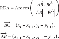
Equation (1) does not indicate the node turning left or right, so we obtain this information by coordinate transform. As Figure 6 shows, in the original coordinate system, the angle between $\overrightarrow{AB}$ and the positive direction of x-axis is α. Now, we take the direction of vector $\overrightarrow{AB}$ as the positive direction of x-axis in the new coordinate system. We can calculate the new coordinates $(x^{\prime },y^{\prime })$ of point C in the new coordinate system by (2). If $y^{\prime }$ of node C is positive, node C turns left; otherwise, it turns right.

$$\begin{array}{cc}& \left(x^{\prime },y^{\prime }\right)=\left(x,y\right)·\left(\begin{array}{cc}\cos \alpha & -\sin \alpha \\ \sin \alpha & \cos \alpha \end{array}\right).\end{array}$$

(2)

Figure 6

Coordinate transform.

4.2. Distribution of Relative Direction Angles

We study the distribution of relative direction angles on a real vehicles mobility trace. The traces we used were collected from a MANET experiment consisting of 240 vehicles. These vehicles traveled over an area of approximately 240 square kilometers near New Jersey, USA, for hours. Each vehicle noted its GPS locations every second. We do not analyze the RDA of synthetic mobility models such as Random Waypoint because the mobility traits of synthetic mobility models are totally different from that of real mobility traces.

We computed the relative direction angle every 10 seconds. Figure 7 shows a vehicle's relative direction angles during 180 minutes. This figure implied that the vehicle turned its original direction to left or right within a narrow range during most of the experiment time. Rarely the mobile vehicle turned its direction sharply. Besides, the times that the vehicle turned left roughly equaled to the times it turned right.

Figure 7

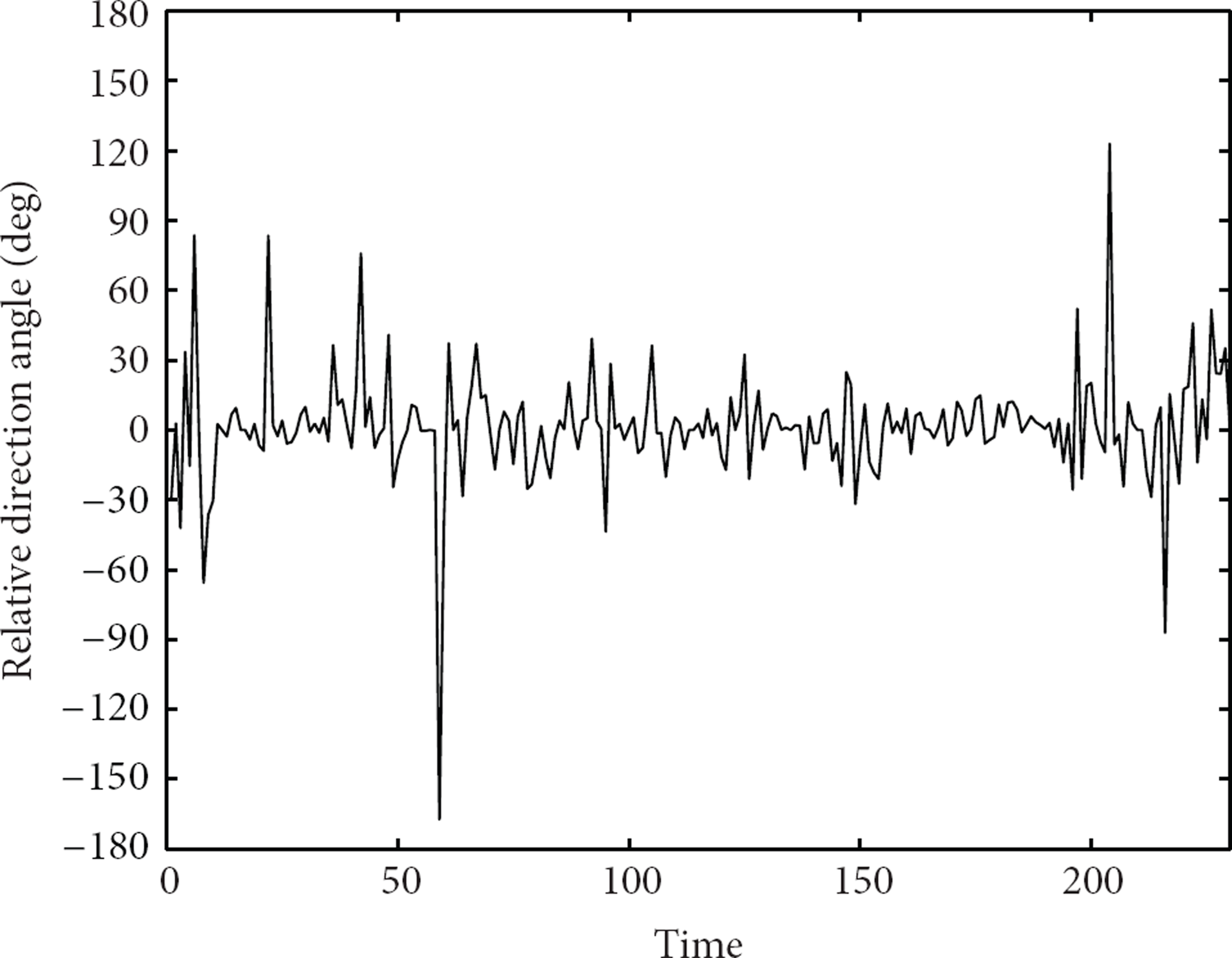
A vehicle's relative direction angle variation.

Then, we study the RDA distribution of all the vehicles. Table 1 depicts the distribution of absolute relative direction angle during the whole 180 minutes. From the statistics we can simply conclude that a mobile vehicle does not select its new direction randomly from a uniform distribution (0°, 180°). Our study shows that over 93% relative direction angles were within a range $[-{30}^{°},{30}^{°}]$ .

Table 1

Distribution of absolute RDA.

Angle	0–30	30–60	60–90	90–120	120–150	150–180
Distribution	93.08%	3.9%	1.73%	0.43%	0.43%	0.43%

5. Vehicle Mobility Prediction

Here, we employ the mobility analysis result that we have made to develop a location prediction algorithm: Triangle And Circle (TRAC). TRAC composes of the location prediction and antenna adjustment. In location prediction step, TRAC predicts a possible circular region, where the moving receiver may enter into in the near future. In antenna adjustment step, the transmitter points its antenna at the predicted circular region and adjusts the beam-width of its directional antenna to cover the predicted region.

5.1. Antenna Assumption

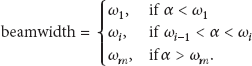
The directional antenna can alter its beam-width, but the beam-widths of the antenna are discrete. The possible beam-widths can only be ${\omega }_i,i=1,2,\dots ,m$ , and ${\omega }_{\mathrm{1}}<{\omega }_{\mathrm{2}}<\cdots <{\omega }_m$ .

5.2. Step 1: Location Prediction

Denote the last two geographical locations of a receiver as $A(x_{i-1},y_{i-1})$ and $B(x_i,y_i)$ , respectively. $(x_{i-1},y_{i-1})$ is the location stored in the neighbor table “history location” field and $(x_i,y_i)$ is the location stored in “current location” field. As illustrated in Figure 8, the distance between the A and B is $d_i$ and the distance from the transmitter (T) to the receiver is $D_i$ . The T (Transmitter) uses the following algorithm to predict a possible region where a receiver moves into.

Figure 8

Point the directional beam to the center of the circle.

• (1)

  Calculate the slope of $\overrightarrow{AB}$ . Let the slope of $\overrightarrow{AB}$ to be k,

  $$\begin{array}{cc}& k_{}=\frac{y_i-y_{i-\mathrm{1}}}{x_i-x_{i-\mathrm{1}}},\hspace{1em}{x}_i\ne x_{i-\mathrm{1}}.\end{array}$$

  (3)

• (2)

  Make an equilateral triangle whose one vertex is at B position and its center $(x_{i+1},y_{i+1})$ is on the extension line of $\overrightarrow{AB}$ as Figure 8 shows. The length of edges of this equilateral triangle is $d_i$ . Calculate the coordinate of the equilateral triangle's center, $(x_{i+1},y_{i+1})$ , by (4),

  $$\begin{array}{cc}& x_{i+\mathrm{1}}=x_i+\frac{\sqrt{\mathrm{3}}d}{\mathrm{3}}\frac{x_i-x_{i-\mathrm{1}}}{\left|x_i-x_{i-\mathrm{1}}\right|}\cos \left(\arctan \left(\left|k\right|\right)\right),\hspace{1em}{x}_i\ne x_{i-\mathrm{1}}\\ y_{i+\mathrm{1}}=y_i+\frac{\sqrt{\mathrm{3}}d}{\mathrm{6}}\frac{y_i-y_{i-\mathrm{1}}}{\left|y_i-y_{i-\mathrm{1}}\right|}\sin \left(\arctan \left(k\right)\right),\hspace{1em}{y}_i\ne y_{i-\mathrm{1}}\\ d=\sqrt{{\left(x_i-x_{i-\mathrm{1}}\right)}^{\mathrm{2}}+{\left(y_i-y_{i-\mathrm{1}}\right)}^{\mathrm{2}}}.\end{array}$$

  (4)

• (3)

  Draw a circle that can contain the equilateral triangle with smallest radius. The circular region is the possible region where the mobile node might move into in near future. The circle and the equilateral triangle have the same center, $(x_{i+1},y_{i+1})$ , and the radius of the circle is $r_i$

  $$\begin{array}{cc}& r_i=\frac{\sqrt{\mathrm{3}}d}{\mathrm{3}}.\end{array}$$

  (5)

5.3. Step 2: Antenna Beam-Width Adjustment

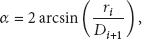
Calculate the needed sector angle α by (6),

$$\begin{array}{cc}& \alpha =\mathrm{2}\arcsin \left(\frac{r_i}{D_{i+\mathrm{1}}}\right),\end{array}$$

(6)

where $r_i$ is calculated by (5) and $D_{i+\mathrm{1}\mathrm{\hspace{0.17em}\hspace{0.17em}}}$ is the distance from the transmitter to the receiver. Since the beam-width of the antenna is discrete, the practical beam-width cannot be more narrow than the needed α. The antenna adjusts its beam-width by (7), and then the transmitter points its antenna at the predicted circular region,

$$\begin{array}{cc}& \text{beamwidth}=\{\begin{array}{cc}{\omega }_{\mathrm{1}},\hfill & \text{if}\hspace{0.17em}\hspace{0.17em}\alpha <{\omega }_{\mathrm{1}}\hfill \\ {\omega }_i,\hfill & \text{if}\hspace{0.17em}\hspace{0.17em}{\omega }_{i-\mathrm{1}}<\alpha <{\omega }_i\hfill \\ {\omega }_m,\hfill & \text{if}\hspace{0.17em}\alpha >{\omega }_m.\hfill \end{array}\end{array}$$

(7)

6. Evaluation

6.1. Metric

The metric we utilize to evaluate the prediction efficiency is prediction accuracy rate. The definition of prediction accuracy rate is the following:

$$\begin{array}{cc}& \text{prediction}\hspace{0.17em}\text{accuracy}\hspace{0.17em}\text{rate}=\frac{{\sum }_{i=\mathrm{1}}^X{x}_i}{X},\mathrm{\hspace{0.17em}\hspace{0.17em}}\\ x_i=\{\begin{array}{cc}1\hfill & \text{if}\hspace{0.17em}\hspace{0.17em}{l}_i\in P_i\hfill \\ 0\hfill & \text{if}\hspace{0.17em}\hspace{0.17em}{l}_i\notin P_i,\hfill \end{array}\end{array}$$

(8)

where $l_i$ is the real location of a node at time i and $P_i$ is the predicted region by TRAC at time i. $l_i\in P$ means the node is within the predicted region P. X is the total times of predictions.

6.2. Parameter Analysis

6.2.1. Influence of Beam-Width

The simulation program randomly selects one position in the experiment area as the transmitter's location where we place a directional antenna to send signals. Then, the simulation program randomly selects a vehicle in the New Jersey traces as the receiver. It calculates the average probability of a receiver being within the transmitters' directional beam during 180 minutes. To make the experiment more credible, we further repeat the experiment 50 times and use the average value. We assume the heartbeat cycle is 10 seconds.

First, we study the influence of beam-width on the prediction accuracy rate. Figure 9 shows the algorithm prediction accuracy rate with different antenna beam-widths. As we can see from Figure 9, if an antenna's beam-width is as narrow as 2°, the prediction accuracy rate is less than 0.7. This is reasonable because if the beam-width is too narrow to cover the possible region where the mobile vehicle might move into as Figure 8 shows the prediction accuracy rate is low. On the other hand, when the beam-width is wider than 10°, the prediction accuracy rate is almost constant. If most of the predicted circular regions are already covered by a 10° beam-width directional beam, the prediction accuracy rate does not increase even if we further increases the antenna's beam-width.

Figure 9

Average prediction accuracy rate under different beam-widths (heartbeat cycle = 10 sec).

6.2.2. Influence of Beam-Width

Then, we study the influence of heartbeat cycle on the prediction accuracy rate. Figure 10 shows the prediction accuracy rates with different heartbeat cycles when the beam-width being 10°. This figure shows that with the increasing of the heartbeat interval, the predicting performance decreases. When the interval between two heartbeat packets is long, the probability of a vehicle travelling along its previous direction decreases because roads are not straight always. The distance that a vehicle travels during a long interval differs much more than during a short interval. Therefore, we suggest that the heartbeat cycle is not longer than 10 seconds.

Figure 10

Average prediction accuracy rate under different heartbeat cycles (beam-width = 10°).

We study the reason of the decrease of the prediction accuracy rate shown in Figure 10. In the above evaluation simulation, the average distance from the sender to a receiver was about 3000 meters. We can calculate the value of r based on Figure 11.

Figure 11

Illustration of computing r. $\tan (\omega /\mathrm{2})=r/D,\hspace{0.17em}r=D·\tan (\omega /\mathrm{2})$ . Assume D = 3000 m and ω = 10°, then $r=262$  m.

Assume that a vehicle's average speed is 90 km/hour, then the vehicle can exercise 250 meters in 10 seconds and run 500 meters in 20 seconds and 750 meters in 30 seconds. When the heartbeat cycle is 10 seconds, a vehicle averagely travels 250 meters during a heartbeat cycle. So, it hardly runs out of the predicted region with $r=262$ meters, and the algorithm prediction accuracy rate is about 96%. When the heartbeat cycle is 20 seconds, vehicles can run 500 meters during a heartbeat cycle and the probability of the car running out of the predicted region with $r=262$ meters improves. Then, the prediction accuracy rate of TRAC is down to 50%. When the heartbeat cycle is 30 seconds, cars in a heartbeat cycle average runs 750 meters. As the probability of the car running out of the predicted region is very high, the prediction accuracy rate of TRAC is only 34%.

6.3. Validation

Next, we validate our prediction algorithm on other traces. The traces we employed to validate our algorithm is generated by Communication Systems Group (CSG), ETH Zurich (http://www.csg.ethz.ch/). The validation simulation is made in a 3000 m*3000 m square area for 1 hour. The antenna beam-widths are 5° and 10°and the heartbeat cycle is 10 seconds. The location of the transmitter is randomly selected within the simulation area. For simplicity, we assume the transmitter is immobile. To make the validation more confident and accurate, we did the simulation 50 times on every mobility trace.

Figure 12 traces that a vehicle moved in rural terrain road network, urban terrain road network, and city terrain road network. As there are more and more roads from rural to urban and city, a vehicle has more and more direction selections and road selections.

Figure 12

(a) vehicle trace in rural terrains, (b) vehicle trace in urban terrains, and (c) vehicle trace in city terrains.

Figure 13 shows the prediction accuracy rates of TRAC on the rural, urban, and city traces. The prediction accuracy rates are ordered from small to large. From the figure, we can find that the lowest prediction accuracy rate is higher than 0.88 and the prediction accuracy rates on city were lower than those on the other two traces mostly. So, the algorithm accuracy depends on the terrain where the vehicle travels.

Figure 13

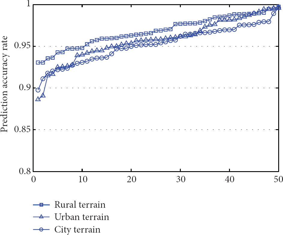
Prediction accuracy rates in the rural, urban, and city terrains.

Further, we validate the mobility prediction algorithm on mobility models: Random Waypoint and Manhattan Model. The simulation of mobility model is also made in a 3000 m*3000 m square area for 1 hour. Figure 14(a) is the traces by Random Waypoint model, and Figure 14(b) is the trace by Manhattan Model, which are generated by ETH Zurich CSG mobility generator.

Figure 14

(a) Random Waypoint Model trace and (b) Manhattan Model trace.

Figure 15 shows the prediction accuracy rates of TRAC on the Random Waypoint and Manhattan Model. The prediction accuracy rates are ordered from small to large. Most of the prediction accuracy rates on Manhattan Model trace are lower than that on Random Waypoint trace because in Manhattan Model, nodes turned their directions frequently and all the relative direction angles were 90°.

Figure 15

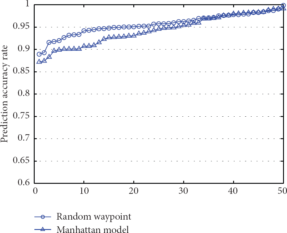
Prediction accuracy rates on mobility models.

Figure 16 shows the average prediction accuracy rates on above traces. The average prediction accuracy rate on the New Jersey vehicles traces is 95.3%. The average prediction accuracy rate on rural road is 96.83%, on urban road is 95.77% and on city road is 95.24%. The increase of road choice brings more unpredictable direction variation during a vehicle's movement, so it is more difficult to predict a vehicle's future location when it travels in city than when it travels on rural road. Thus, the prediction accuracy rate decreases slightly with the increase of road density from rural terrain to city terrain. The prediction accuracy rate on Manhattan Model is the lowest because nodes in Manhattan mobility model often turn left or right 90°. The average prediction accuracy rate on the traces of vehicles on roads is 96%.

Figure 16

Prediction accuracy rates on different mobility traces.

6.4. Performance Evaluation

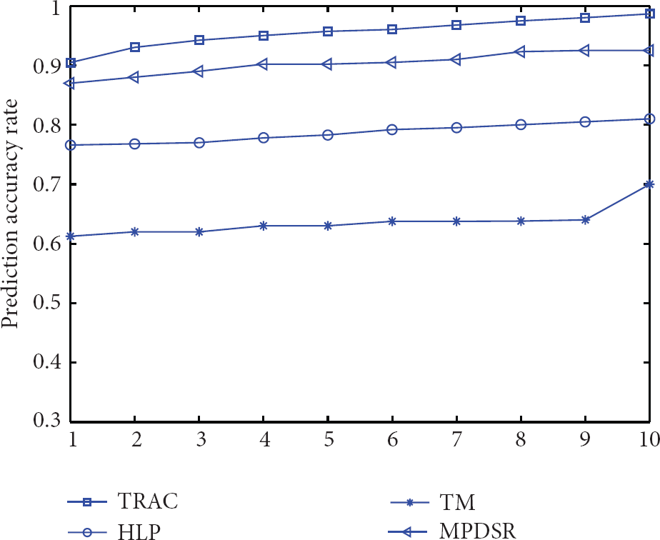
We compare the prediction performance of TRAC with hierarchical location prediction (HLP) algorithm [8], mobility prediction based on dividing sensitive ranges (MPDSR) [9], and mobility prediction based on Transition Matrix (TM) [10]. The values of the parameters for HLP, MPDSR, and TM were assigned to make the prediction accuracy rate of them to be high. To make the experiment more credible, we did the simulation 10 times. Figure 17 shows the prediction accuracy rates of TRAC, HLP MPDSR, and TM. As we can see, the prediction accuracy rates of TRAC are higher than those of the other three.

Figure 17

Prediction accuracy rates on different mobility traces.

HLP, MPDSR, and TM need a mobile node's history traces to study their possible mobility sequences and to match its current mobility sequence with these mobility sequences to find the node's next possible location or cell. These algorithms cannot be applied in real-time prediction when nodes are traveling in a strange area. The largest advantage of TRAC is that it does not need a node's history mobility traces to study its mobility pattern. So, TRAC algorithm can be employed to predict a mobile node's next region real-timely even if it is traveling in a new area.

The validation and evaluation results show that the prediction accuracy rate of TRAC is usually higher than 96%, and the TRAC is independent of the New Jersey trace and can be applied in other applications.

7. Conclusions

In this paper, we study the location prediction issue for communications between vehicles and vehicle to infrastructure using directional antennas. To do this, we analyzed a real trace and extracted the direction characteristic from it. We found most of the relative direction angle is in the range of (−30°, 30°). Based on this mobility analysis result, we propose a location prediction algorithm. The algorithm predicts a possible circular regain where the vehicle might move into in the next period. To validate the location prediction algorithm, we apply the algorithm on three GIS-based road network traces and two random mobility models traces. Experiment results show the average algorithm prediction accuracy rate is as high as 96%. We also studied the influence of different antenna beam-widths and interval durations on the algorithm accuracy. The largest advantage of TRAC is that it does not need a vehicle's history mobility traces to study its mobility pattern and it can be applied in real-time prediction when vehicles travel in a strange area.