Sage Journals: Discover world-class research

Abstract

Topology optimization provides great convenience to designers during the designing stage in many industrial applications. With this method, designers can obtain a rough model of any part at the beginning of a designing stage by defining loading and boundary conditions. At the same time the optimization can be used for the modification of a product which is being used. Lengthy solution time is a disadvantage of this method. Therefore, the method cannot be widespread. In order to eliminate this disadvantage, an element removal algorithm has been developed for topology optimization. In this study, the element removal algorithm is applied on 3-dimensional parts, and the results are compared with the ones available in the related literature. In addition, the effects of the method on solution times are investigated.

1. Introduction

In a designing stage, one of the most difficult problems that designers have to overcome is the balancing of “trade-offs.” In the design of a structural component, there is a trade-off between weight and strength. When the weight of the component is decreased, the strength of the component is also decreased. But the designer must find the minimum weight and sufficient strength combination for the design component. Because the weight is known to be one of the main factors of the final cost of load-carrying structures, the weight reduction is often set as the main objective of the designing task. Topology optimization is a useful tool for a designer which generates the optimal initial shape of a mechanical structure. The structural shape is generated within a predefined design space. In addition, the user defines structural supports and loads. Without any further decision and guidance of the user, the method will give the structural shape thus providing a first idea of an optimum geometry. A desired property of the structure is maximized by changing the shape of the given material. Usually this maximized property is stiffness. Another usage of topology optimization is minimizing the weight, subjected to a given constraint (such as stress) [1].

Topology optimization is used for many different engineering applications such as thermodynamic problems [2 –4], fluid mechanics [5, 6], electro mechanics [7, 8], acoustic problems [9], multiphysics problems [10], and solid mechanics [11, 12]. By using topology optimization, designers can easily solve very difficult and complex problems; hence, usage of this method increases day by day.

The simple idea of the topology optimization is the removal of less efficient materials from a structure. To find accurate solution of topology optimization, the designer must increase the number of iteration and the numbers of elements. When the number of iteration and elements are increased, solution time also increases extremely. This is the main drawback of the method that must be overcome. For this reason, in the optimization processes, passive elements (which are found from FE analyses) were eliminated after every iteration loop in a previous study [1]. In the subsequent iteration loop, unnecessary elements were not used during solution. Hence, at each progressive solution loop, the number of elements decreased. The algorithm is developed for 2D parts with considerable time saving compared with other methods. In this study, previously developed element removal algorithm for 2D models [1] is improved for 3D models.

2. Element Removal Method

The main idea of the topology optimization is THE removal of ineffective (comparatively small stressed) elements from the design domain. Element removal method (ERM) is developed to systematically remove low-density elements from the design domain [13]. Bruns and Tortorelli [13] developed an element removal and reintroduction strategy for topology optimization method. Material density method is used to decide which element IS to be removed or reintroduced. For the smoothness of the design domain, weight function is calculated. In this function, all elements are used to calculate weight of each element. This causes high CPU usage, especially with high element numbers. To overcome this drawback, in the optimization processes, passive elements (which were found from FE analyses) were eliminated after every iteration loop in a previous study [1]. In the next iteration loop, unnecessary elements are not used during solution. Hence, at each progressive solution loop, the number of elements is decreased. The algorithm is developed for 2D parts with considerable time saving. In this algorithm, ineffective elements are selected according to their stress values which are calculated from FEA. FEA is applied on the design domain in a loop and after every analysis; elements with lowest stress values are deleted. In the proposed algorithm, reintroduction of the removed element does not exist. After the removal operation elements are renamed to put the remaining elements in an order. Then these elements form the new design domain for the next step of the loop, and a new optimization step starts. The optimization cycle stoppes when volume-reduction ratio or yield stress is reached to predefined values. The optimization process will be faster at every subsequent cycle as the ineffective elements are not used in the following FEA solutions. Therefore, total solution time decreases rapidly. By using this method, 90% time reduction is obtained for statically loaded 2D planer machine parts [1].

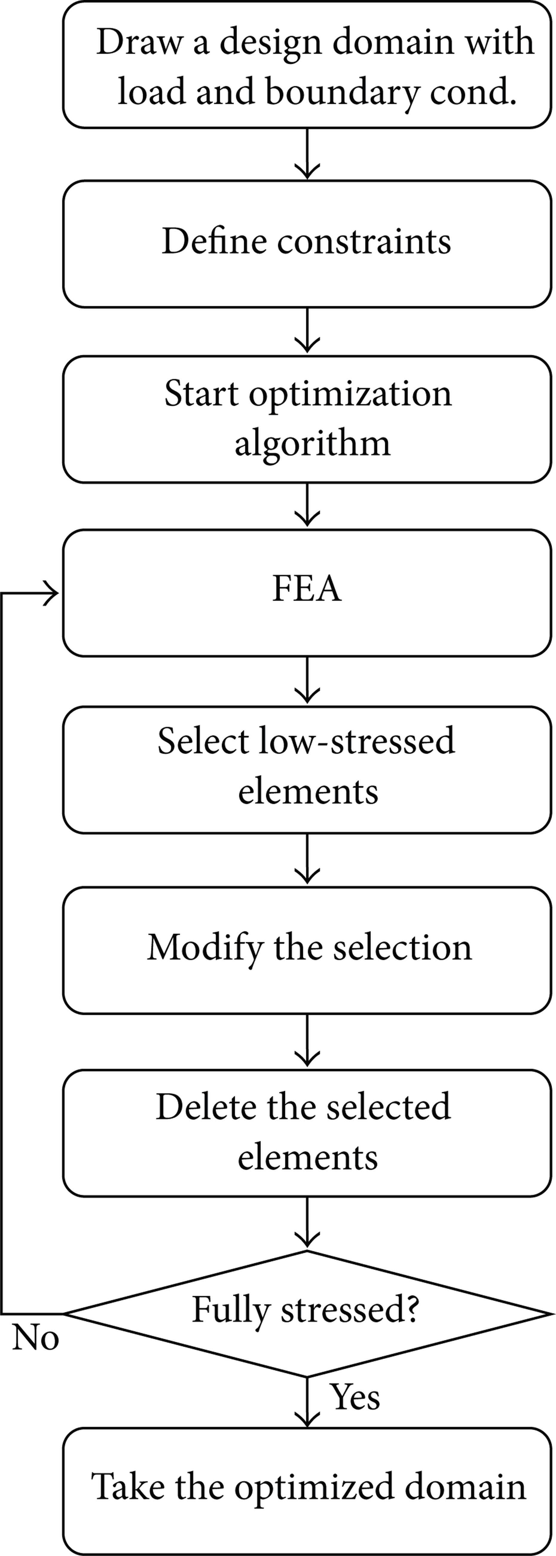
In Figure 1, a schematic view of optimization process with ERM can be seen. According to this procedure, the design domain must be drawn with load and boundary conditions. Then, the constraints (allowable stress and volume reduction ratio) are defined. After the definition of constraints, the optimization process can be started. In the optimization process, firstly FEA is performed and the low stressed elements are selected. Then, the modification algorithm is applied to obtain fine material distribution. After that, the selected elements are deleted from the design domain and they are not used in the subsequent iteration loops. Finally, constraints are checked; if one of the constraints is reached, optimization loop is ended, if not, the loop continues. This algorithm is written as a macro in ANSYS FEA program.

Figure 1:

ERM procedure.

During the application of the ERM, a modification algorithm is used to prevent porous structure during element removal. In the modification algorithm, by checking the neighbors of the selected element to be deleted (in Figure 2), the algorithm decides whether or not to delete the selected element.

Figure 2:

Selected element and its neighbours.

Developed algorithm can be applied on a simple prism. In Figure 3, a 3D design domain with loading and supporting conditions is given. Unit load is applied at midpoint of upper surface of the design domain, and fixed support is applied at lower corners. In Figure 4, some of the ineffective elements are removed from the design domain after some iteration loops. The final optimized domain can be seen in Figure 5.

Figure 3:

Design domain with 250 elements.

Figure 4:

Middle step of the ERM.

Figure 5:

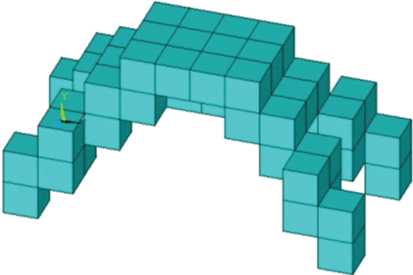
Optimized model with ERM.

Figure 5 is the final optimization result with minimum material usage, and at the same time, stress values are in the acceptable limits. In the present study, an algorithm based on the element removal is developed to optimize parts for minimum material usage. The key point of the algorithm is the removal of less effective elements from the design domain. Initial models such asthose given in Figures 3 –5 are encouraging for effectiveness of the algorithm.

3. Results and Discussions

The validation of the proposed algorithm is discussed in this section. The results of the present study are compared with those obtained from therelated literature. There are two steps as follows.

Comparing results of the ERM with those of the literature.

Comparing solution times of the ERM with those of Ansys.

3.1. Comparison with the Literature

In this section, ERM is compared with the literature. The aim of this section is to discuss the validity of the proposed ERM. For comparison, three different examples are used. In these examples, solid elements are used for mesh and structural steel is used as material. Load is considered to be unit load.

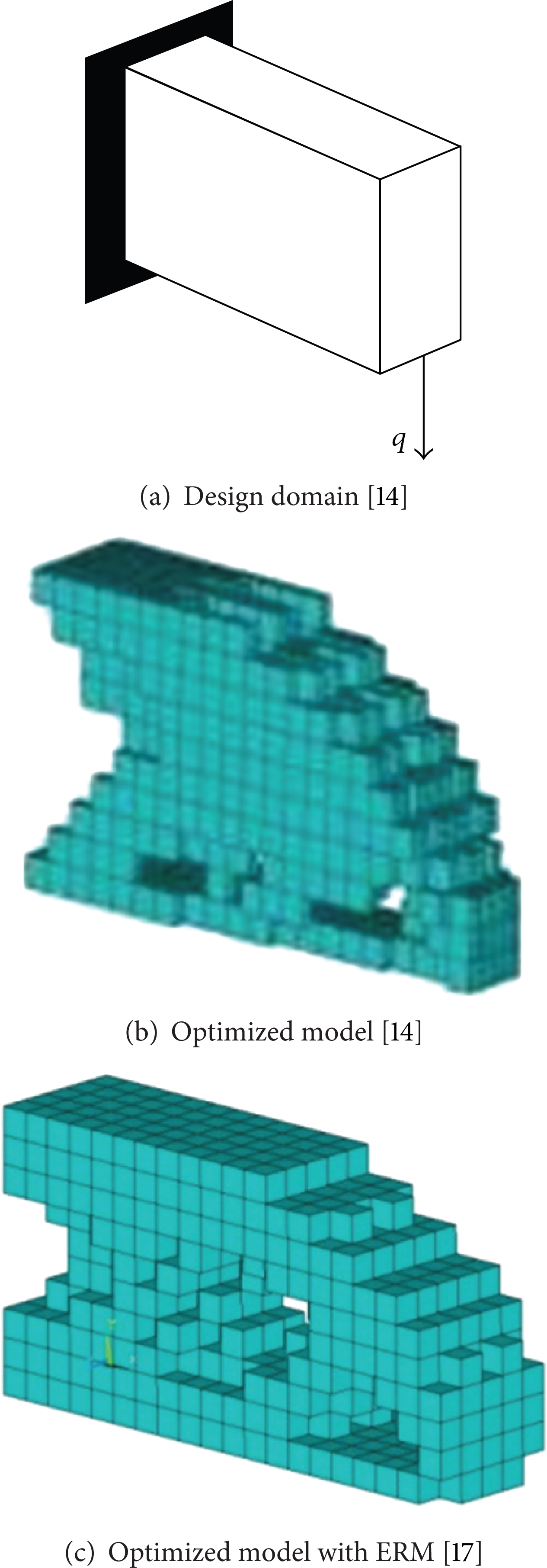
In the first example, a cantilever beam (in Figure 6 (a) [14]) whose one end is fixed and the other end is center loaded is optimized. Volume reduction is used as 50% for constraint. The literature result is shown in Figure 6 (b) [14], and ERM result can be seen in Figure 6 (c).

Figure 6:

Center-loaded cantilever beam model.

In the second example, a cantilever beam (in Figure 7 (a) [14]) whose one end is fixed and the other end lower edge is loaded is optimized. Volume reduction is used as 70%. The literature result can be seen in Figure 7 (b) [14], and element removal result can be seen in Figure 7 (c).

Figure 7:

End-lower-edge-loaded cantilever beam model.

In the third example, an L-shaped beam (in Figure 8 (a) [14]) which is loaded as shown in Figure 8 (a) is optimized. Volume reduction ratio is used as 50% for constraint. The literature result can be seen in Figure 8 (b) [14], and element removal result can be seen in Figure 8 (c).

Figure 8:

L-shaped beam model.

The results can be compared only visually because there are no numerical results in the literature. When the results are compared visually, outcomes of the present study are nearly the same that of as given in reference. These results imply that the developed algorithm is working well.

After the validation of the algorithm, its advantages can be investigated. For this investigation, solution times are compared in the next part.

3.2. Comparison of Solution Times

Main disadvantage of the topology optimization is that a lengthy solution time is required. For a machine part (such as connecting rod and suspension arm), designers must use high element numbers to obtain better results. Increased element numbers yield asymptotically increased solution time. One of the advantages of the proposed ERM is shorter solution time. Solution times of the proposed ERM algorithm and ANSYS topology optimization tool are compared in this part. For this comparison, two design domains (Figures 9 and 14) are meshed using different element numbers.

Figure 9:

The design domain with 2000 elements for Case 1 (3D schematic view).

A computer with 2.13 GHz dual core CPU, 2 GB ram, and 160 GB hard disk is used for solutions. Volume reduction is taken as 80% for both ERM and ANSYS. Iteration number is taken as 37 for ANSYS.

Case 1. Solid elements are used to mesh the design domain, structural steel is used as material (modulus of elasticity (E) = 200 GPa, Allowable stress (σ_a) = 150 MPa), and 21 kN load is applied as shown in Figure 9. The results can be seen in Figure 10 for this case. As well as comparing the solution times, outcomes of the optimizations are also compared; for this aim maximum stress and deformation values are shown in Figures 11 and 12. Comparison of the solution times can be seen in Figure 13. All results are tabulated in Table 1 for the ease of comparison.

Table 1:

Results of ERM and ANSYS for Case 1.

	Element number	Iteration number	Solution time (sec)	Time reduction (%)	Deformation (mm)	Von-Mises stress (MPa)

Ansys	2000	37	379	58.6	0.422	133
ERM	2000	37	157	58.6	0.247	98
Ansys	4225	37	1203	63.8	0.265	113
ERM	4225	37	436	63.8	0.232	85
Ansys	6525	37	2575	65.2	0.334	121
ERM	6525	37	896	65.2	0.218	80
Ansys	7936	37	4470	70.8	0.280	118
ERM	7936	37	1307	70.8	0.193	81
Ansys	9826	37	6800	73.0	0.274	133
ERM	9826	37	1835	73.0	0.217	87
Ansys	16000	37	15370	74.4	0.240	111
ERM	16000	37	3939	74.4	0.183	92
Ansys	23805	37	31930	75.7	0.197	103
ERM	23805	37	7771	75.7	0.190	94
Ansys	35146	37	77433	75.5	0.228	121
ERM	35146	37	18989	75.5	0.185	119
Ansys	48778	37	137970	68.5	0.286	137
ERM	48778	37	43467	68.5	0.183	131

Figure 10:

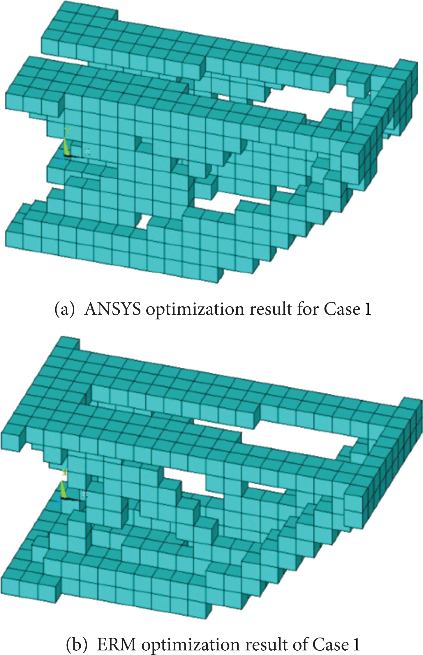
Visual comparisons of ANSYS and ERM results for Case 1.

Figure 11:

Maximum stress values of different element numbers for Case 1.

Figure 12:

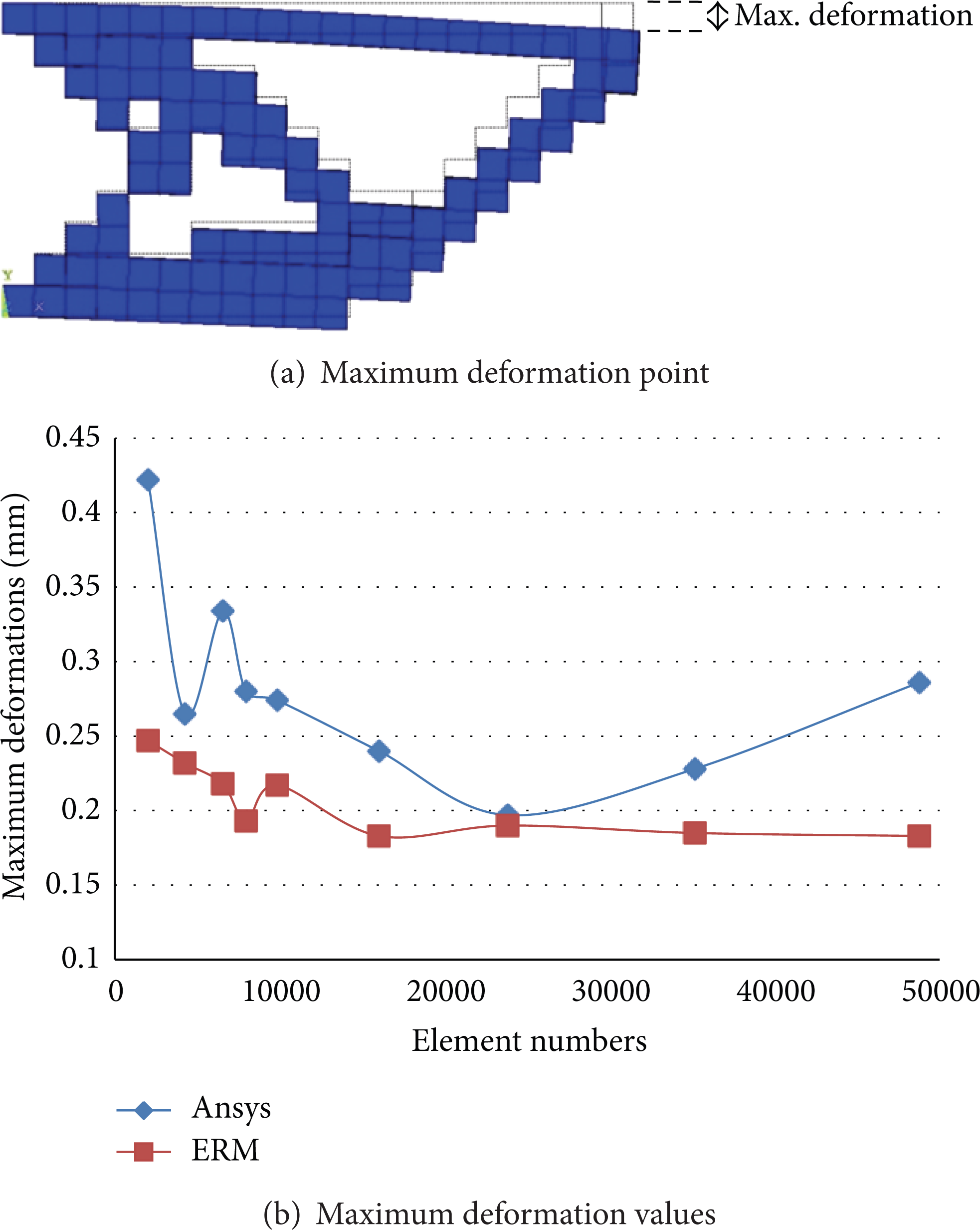
Maximum deformation values of different element numbers for Case 1.

Figure 13:

Solution times of different elements number for Case 1.

Figure 14:

Design domain with 4000 element for Case 2 (3D schematic view).

Case 2. Solid elements are used to mesh the design domain, structural steel is used as material (E = 200 GPa, σ_a = 150 MPa), and 10 kN load is applied as shown in Figure 14. The result of the optimization is shown in Figure 15. Maximum stress and deformation values are shown in Figures 16 and 17 for different element numbers. Comparison of the solution times can be seen in Figure 18. All the results are tabulated in Table 2.

Table 2:

Results of ERM and Ansys for Case 2.

	Element number	Iteration number	Solution time (sec)	Time reduction (%)	Deformation (mm)	Von-Mises stress (MPa)

Ansys	2048	37	388	58.5	0.058	17.1
ERM	2048	37	161	58.5	0.032	13.7
Ansys	4000	35	1139	63.7	0.032	16.8
ERM	4000	39	413	63.7	0.023	11.8
Ansys	6912	31	2728	65.2	0.069	22.7
ERM	6912	37	950	65.2	0.024	14.0
Ansys	8450	37	4760	70.7	0.069	23.0
ERM	8450	37	1392	70.7	0.022	12.4
Ansys	10976	37	7596	73.0	0.056	22.5
ERM	10976	37	2050	73.0	0.021	11.3
Ansys	16384	37	15739	74.3	0.068	24.4
ERM	16384	37	4034	74.3	0.020	11.1
Ansys	23328	37	31290	75.6	0.047	22.9
ERM	23328	37	7616	75.6	0.020	14.2
Ansys	37044	37	63818	72.5	0.048	24.2
ERM	37044	37	17580	72.5	0.020	12.1
Ansys	48668	37	104118	71.9	0.041	21.2
ERM	48668	37	29255	71.9	0.020	13.1

Figure 15:

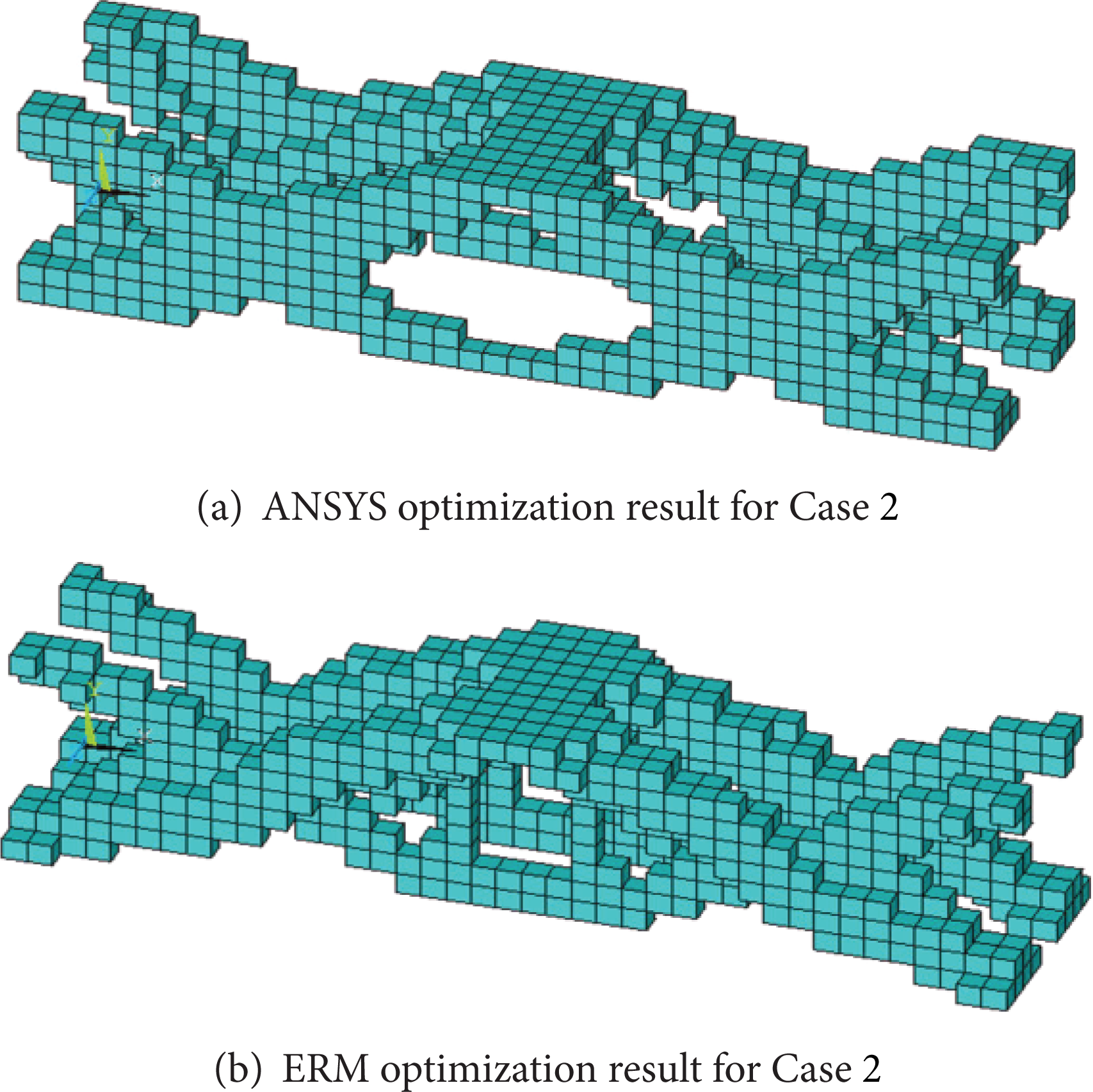
Visual comparisons of ANSYS and ERM results for Case 2.

Figure 16:

Maximum stress values of different element numbers for Case 2.

Figure 17:

Maximum deformation values of different element number for Case 2.

Figure 18:

Solution times of different element number for Case 2.

Investigating Figures 11 and 16 for stress results, some variation in stress value is observed for different element numbers, which is mainly due to local stress concentrations. According to the outcomes, ERM yields lower stressed optimization result even at low element numbers. This outcome implies that stress concentrations are prevented during element removal operations by ERM. Comparing the solution times from Figures 13 and 18 and also in Tables 1 and 2, the advantage of the proposed ERM method is clearly observed for high element numbers especially above 25000 elements. Use of the ERM will yield up to 75% less solution time for topology optimization of a part.

3.3. Applications

The proposed ERM algorithm is applied on two applications. One of them is connecting rod and the other one is suspension arm. The results of the ERM and stress comparisons are given in this part. In both applications, the aim is decreasing the stress values of both parts with the same material usage. Hence, rough design domains are produced using ERM, and final volume is always the same as that of the original part.

Connecting Rod. Connecting rod (Figure 19 [15]) is optimized by using ERM. For this purpose, a design domain is produced with a rough model of rod (Figure 20). Point A is fixed and two load cases (tension and compression loads) are applied at point B. AISI 1045 is used as material (E = 200 GPa, σ_a = 200 MPa). FE model is produced by using tetrahedral solid elements under the given load cases. ERM is applied on this FE model. Outcome of the optimization process can be seen in Figure 21. After the optimization, the optimized domain is remodeled (Figure 22) and analyzed.

Figure 19:

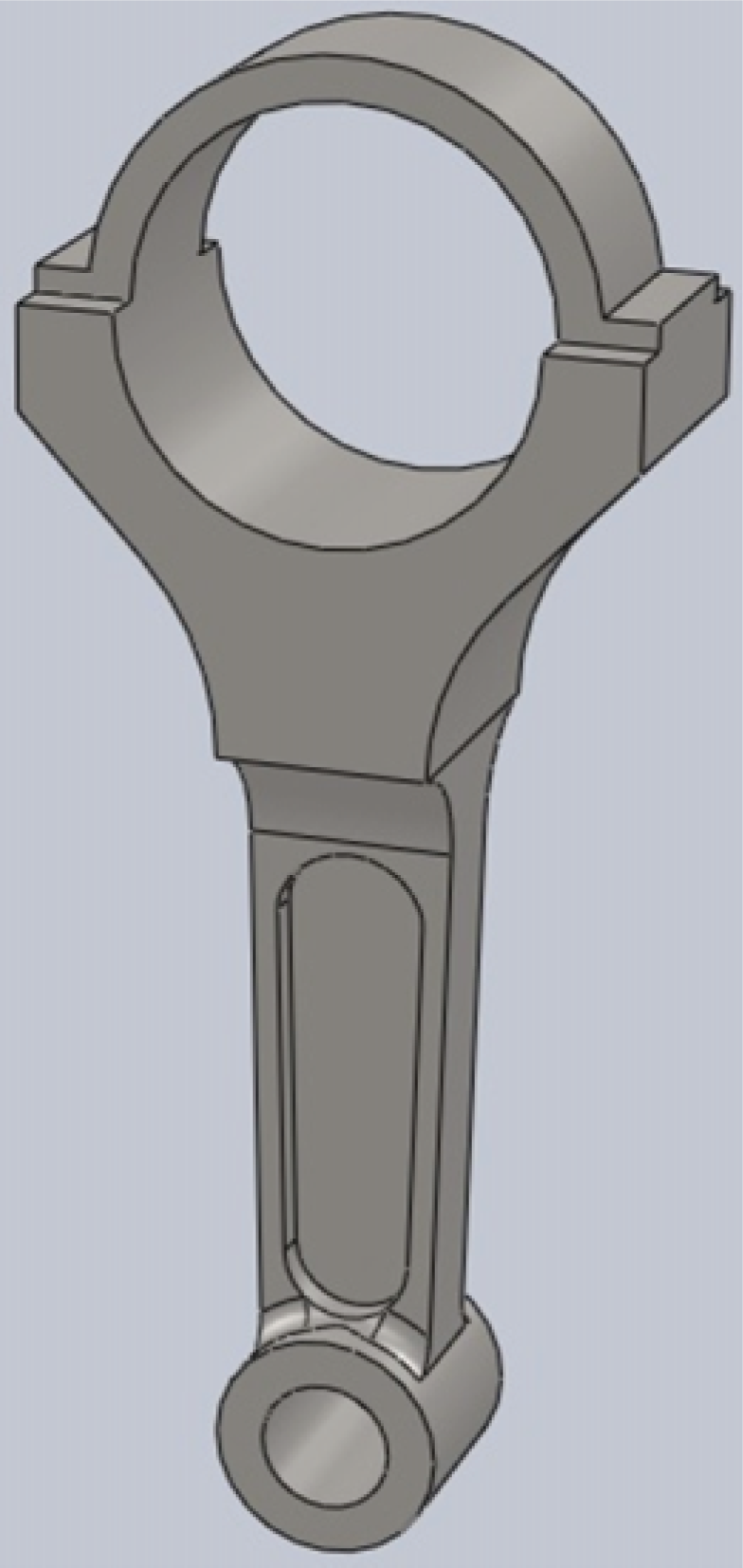
Solid model of original connecting rod [15].

Figure 20:

Design domain of connecting rod.

Figure 21:

Optimization result of connecting rod.

Figure 22:

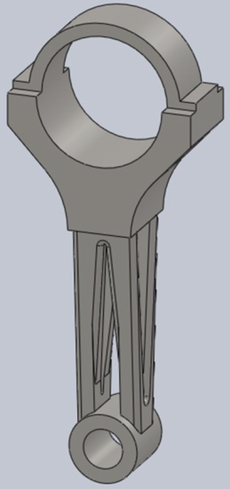
Solid model of optimization result of connecting rod.

ERM algorithm, which is given in Section 2, is used for optimization process. Volume is used as constraint and it is taken as original model's volume, representing equal material usage. After the optimization process, the shape in Figure 21 is obtained.

For analysis, solid model of the above result is produced as shown in Figure 22. After producing the solid model, analysis is performed on the original model and the optimized model. Von-Mises stress distributions of the original and optimized models are given in Figures 23 and 24, respectively.

Figure 23:

Stress result of original model.

Figure 24:

Stress result of optimized model.

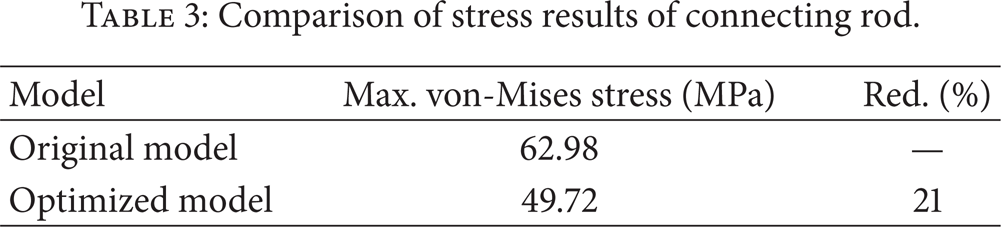
The maximum von-Mises stress result, for the original model in Table 3, is about 63 MPa. For the optimized model, the maximum value is about 50 Mpa. Stress reduction by the use of ERM is about 21%.

Table 3:

Comparison of stress results of connecting rod.

Model	Max. von-Mises stress (MPa)	Red. (%)

Original model	62.98	—
Optimized model	49.72	21

Suspension Arm. In the second case, a suspension arm (Figure 25 [16]) is optimized by using ERM. The original arm is modeled before optimization (Figure 26), then the design domain is modeled (Figure 27) slightly larger than the original model. Points A and B are fixed and load is applied at point C (X = – 25 N, Y = 277 N, and Z = 49 N). FE model is produced by using tetrahedral solid elements under the given load cases. ERM is applied on this FE design domain. Optimization result of the arm is shown in Figures 28 and 29. Then the optimized domain is remodeled (Figures 30 and 31) and analyzed.

Figure 25:

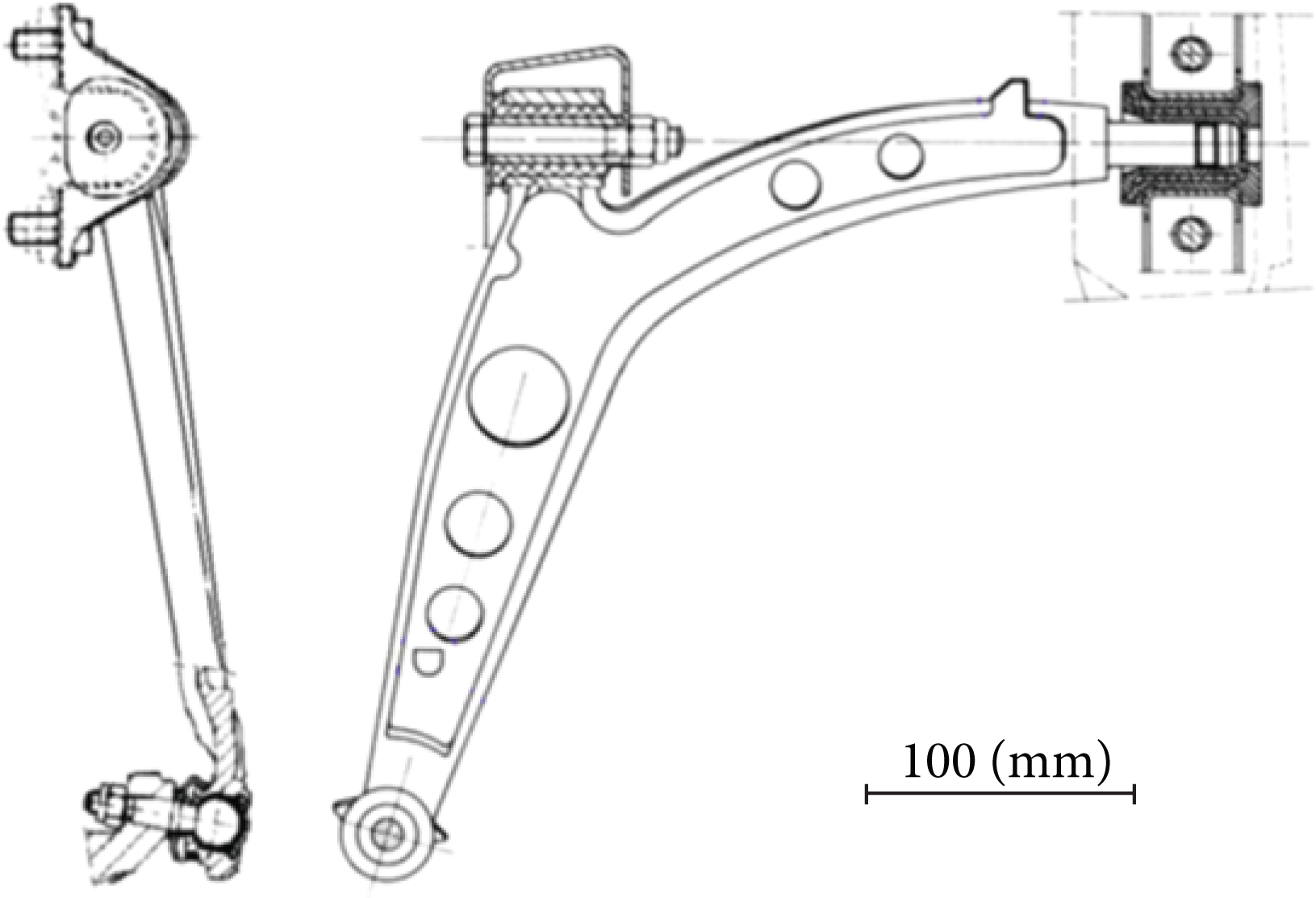
Front and side views of suspension arm [16].

Figure 26:

Solid model of original suspension arm.

Figure 27:

Design domain of suspension arm.

Figure 28:

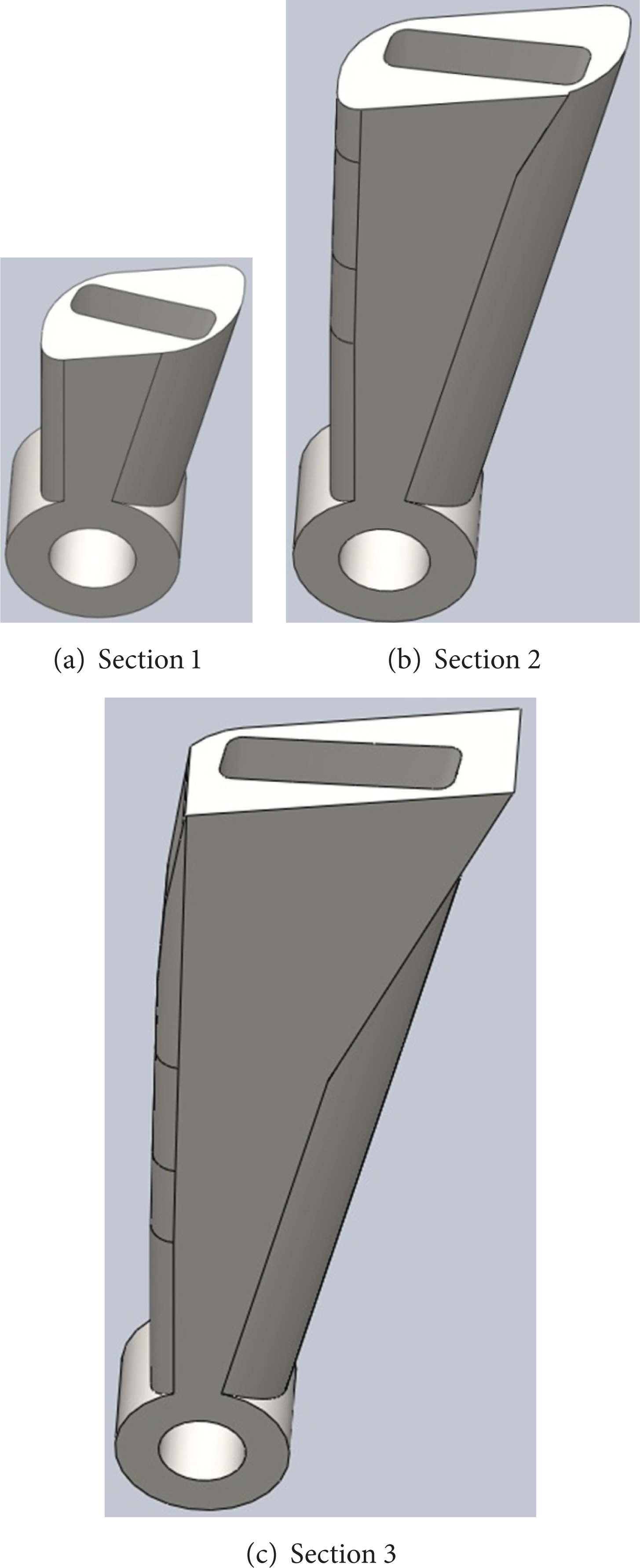
Optimization result of suspension arm.

Figure 29:

Sectional view of optimization result.

Figure 30:

Solid model of optimization result of suspension arm.

Figure 31:

Sectional view of solid model.

For the optimization processes, ERM algorithm, which is given in Section 2, is used. Volume constraint is defined to obtain the same volume as that of the original model. After the optimization process, the shape in Figure 28 is obtained.

Three sections are given in Figure 29 to investigate the interior part of the model. According to the result of optimization, the new model is drawn as shown in Figure 30. Sectional view of this new model can be seen in Figure 31. Analysis is performed on the original model and the optimized models for comparison of their performances. Their von-Mises stress results are given in Figures 32 and 33, respectively.

Figure 32:

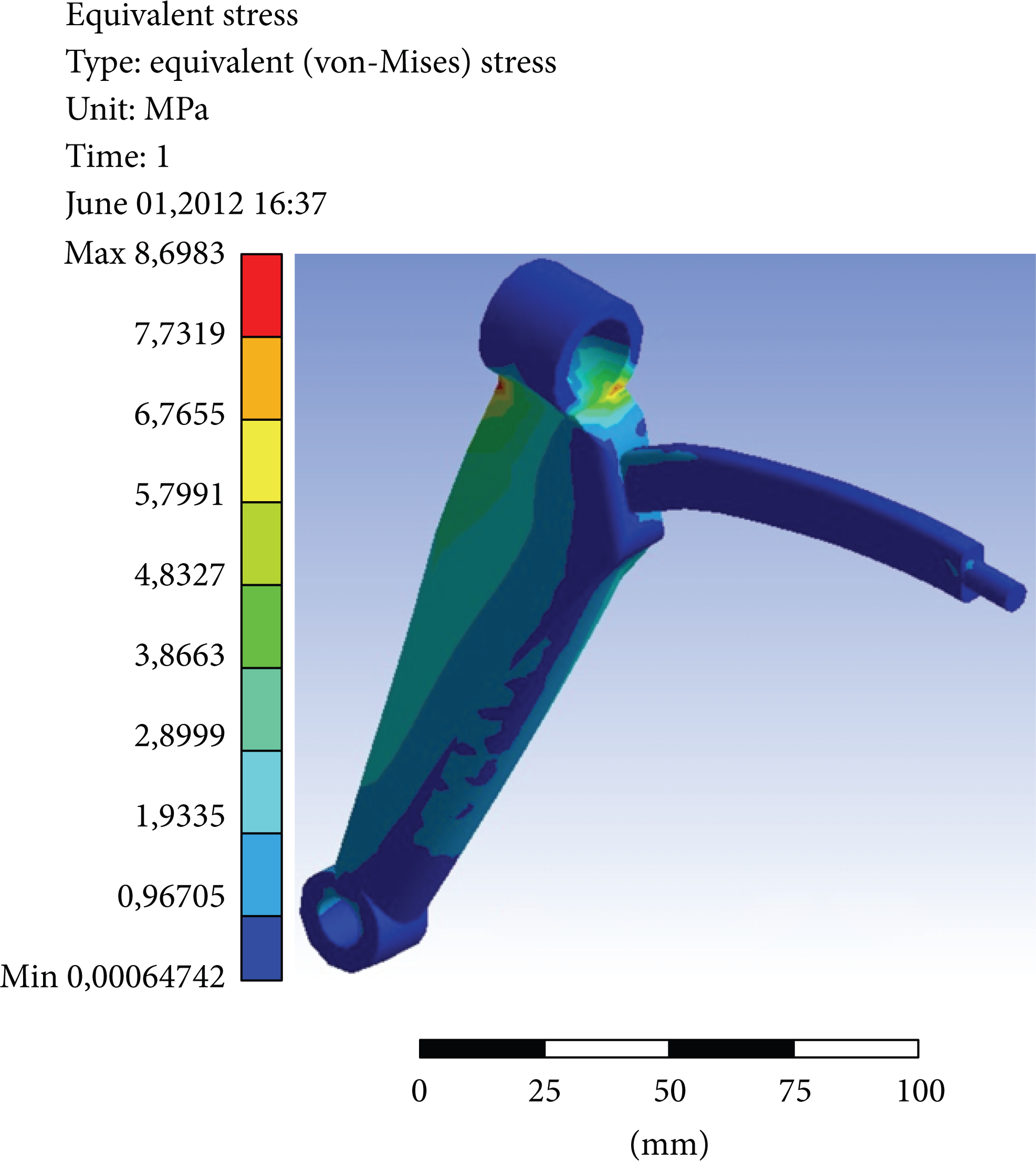
Stress result of original model of suspension arm.

Figure 33:

Stress result of optimized model of suspension arm.

In Table 4, von-Mises stress results for the original and the optimized models are given; about 38% stress reduction is obtained by the use of the proposed ERM.

Table 4:

Comparison of stress results of suspension arms.

Model	Max. von-Mises stress (MPa)	Red. (%)

Original model	14.138	—
Optimized model	8.698	38.48

4. Conclusions

In this study, a new algorithm is developed for topology optimization of 3D machine parts. Validity of the algorithm is proved by means of simple beam parts and two parts from industrial application. The results of the comparisons imply that the element removal algorithm can be safely used for 3D machine parts. Also solution times are compared with ANSYS, and up to 75% time reduction is obtained by using the element removal algorithm. When the stress and deformation results are compared, up to 50% reduction can be obtained depending on the boundary conditions in the ERM results.

References

Göv

İ.

, Applying topology optimization to design of planer machine parts [M.S. thesis], The Institute for Graduate Studies in Natural and Applied Sciences, Gaziantep University, 2009.

Zhuang

Xiong

, and Ding

, “A level set method for topology optimization of heat conduction problem under multiple load cases,” Computer Methods in Applied Mechanics and Engineering, vol. 196, no. 4–6, pp. 1074–1084, 2007.

Fang

, and Tian

, “Thermomechanical compliant actuator design using meshless topology optimization,” in Proceedings of the 7th International Conference on System Simulation and Scientific Computing (ICSC '08), pp. 1018–1025, October 2008.

Yang

, and He

, “Topology optimization of thermal structure based bi-directional interpolation model,” in Proceedings of the International Joint Conference on Computational Sciences and Optimization (CSO '09), pp. 887–890, April 2009.

Guest

J. K.

and Prévost

J. H.

, “Design of maximum permeability material structures,” Computer Methods in Applied Mechanics and Engineering, vol. 196, no. 4–6, pp. 1006–1017, 2007.

Akl

, “Topology optimization of fluid-loaded shells by minimizing the acoustic coupling to the fluid domain,” International Journal of Computational Methods in Engineering Science and Mechanics, vol. 11, no. 6, pp. 337–353, 2010.

Sun

Yang

, “Vibration suppression of a hard disk driver actuator arm using piezoelectric shunt damping with a topology-optimized PZT transducer,” Smart Materials and Structures, vol. 18, no. 6, Article ID 065010, 2009.

Kang

and Luo

, “Non-probabilistic reliability-based topology optimization of geometrically nonlinear structures using convex models,” Computer Methods in Applied Mechanics and Engineering, vol. 198, no. 41–44, pp. 3228–3238, 2009.

Lee

J. W.

and Kim

Y. Y.

, “Topology optimization of muffler internal partitions for improving acoustical attenuation performance,” International Journal for Numerical Methods in Engineering, vol. 80, no. 4, pp. 455–477, 2009.

10.

Yoon

G. H.

and Kim

Y. Y.

, “The element connectivity parameterization formulation for the topology design optimization of multiphysics systems,” International Journal for Numerical Methods in Engineering, vol. 64, no. 12, pp. 1649–1677, 2005.

11.

Xia

Shi

Liu

, and Wang

M. Y.

, “A level set solution to the stress-based structural shape and topology optimization,” Computers and Structures, vol. 90–91, no. 1, pp. 55–64, 2012.

12.

James

K. A.

Lee

, and Martins

J. R. R. A.

, “Stress-based topology optimization using an isoparametric level set method,” Finite Elements in Analysis and Design, vol. 58, pp. 20–30, 2012.

13.

Bruns

T. E.

and Tortorelli

D. A.

, “An element removal and reintroduction strategy for the topology optimization of structures and compliant mechanisms,” International Journal for Numerical Methods in Engineering, vol. 57, no. 10, pp. 1413–1430, 2003.

14.

Hsu

M.-H.

and Hsu

Y.-L.

, “Interpreting three-dimensional structural topology optimization results,” Computers and Structures, vol. 83, no. 4–5, pp. 327–337, 2005.

15.

Gezer

E. Y.

, “Bir mekanizmamn dinamik gerilme analizi,” Graduation project, 2007.

16.

Mrzygłód

and Zieliński

A. P.

, “Multiaxial high-cycle fatigue constraints in structural optimization,” International Journal of Fatigue, vol. 29, pp. 1920–1926, 2007.

17.

Göv

İ.

and Kütük

M. A.

, “Application of element removal method at topology optimization on 3d parts,” in 5th Otomotiv Teknolojileri Kongresi, Bursa, Turkey, June 2010.