A Type of Localization Method Using Mobile Beacons Based on Spiral-Like Moving Path for Wireless Sensor Networks

Abstract

A type of energy optimization localization method with mobile beacon is proposed in this paper. Traverse point of the mobile beacon is marked with the help of the optimum deployment model and the clockwise spiral-like moving path with fixed step size is also established. According to the moving path and the localization time, energy consumption of the network could be estimated and we could also give the sleep scheduling strategy for the node to be localized. Simulation results show that this method could not only promote the accuracy and success rate of localization, but also reduce the energy consumption.

1. Introduction

In Wireless Sensor Networks, sensed data with location information is valuable [1–3]. Several schemes, broadly classified into two categories, have been proposed for dealing with the localization [4, 5]. First, the range-based schemes need either node-to-node distances or angles for estimating locations. The information can be obtained using time of arrival (TOA) [6], time difference of arrival (TDOA) [7], angle of arrival (AOA) [8], and received signal strength indicator (RSSI) technologies [1]. As we know, the range-based schemes typically have higher location accuracy but require additional hardware to measure distances or angles. Second, the range-free schemes do not need the distance or angle information for localization. Although these schemes cannot accomplish as high accuracy as the range-based ones, they provide an economic approach. The representative range-free localization schemes include centroid algorithm [1], DV_HOP algorithm [1], Amorphous localization method [4], APIT algorithm [5] as well as HOP-TERRAIN method [5].

However, the accuracy of current algorithms is mostly environmentally sensitive which leads to low reliability and low success rate about the location results [7, 9]. Meanwhile, locating with the help of fixed beacons will cause the following problems.

First, the network overhead will be increased since the unknown nodes should be directly adjacent to the beacons in order to acquire their location information which leads to high density of nodes.

Second, the communication overhead in localization is larger. The unknown nodes are often in listening mode during the localization process which increase the energy consumption.

Third, to enhance the accuracy of localization, it is necessary to deploy more beacons in the network. However, the more beacon nodes it uses, the greater the overhead layout of the entire network is.

2. Related Works

Therefore, more and more algorithms are proposed to acquire the position information of unknown nodes in wireless sensor networks with the help of mobile beacon, which becomes available with the rapid development of various related research area such as automation and aviation [10–13]. The mobile beacon could be equipped with powerful computational ability to find a result in a very short time which is close to real-time and it could move flexibly according to the motivation it depends on to place human cannot reach. Therefore, diverse algorithms are designed to drive mobile beacon to work on field of Wireless Sensor Networks, but as a primary prerequisite, localization is the first step.

A framework of mobile beacon based localization method is proposed in [11]. Three mobile beacons traverse the field as a group in the shape of isosceles right triangle which enables all the unknown nodes inside the triangle to be localized by receiving three beacon messages. However, it is difficult for these mobile beacons to work synchronously.

Tilak et al. [14] study the time interval for broadcasting of the mobile beacon and propose an adaptive and predictive protocols that control the frequency of localization based on sensor mobility behavior.

Bergamo and Mazzini [15] propose a scheme to perform localization, based on the estimation of the power received by only two beacons placed in known positions. By starting from the received powers, eventually averaged on a given window to counteract interference and fading, the distance between the sensor and the beacons is derived. However, the accuracy of this method is not high.

A type of node localization based on mean shift and joint particle filter is proposed in [16] which improves the accuracy of particle state estimation and reduces the necessary number of samples by using the current observations in sampling procedure to obtain a sample distribution. In addition, Juan et al. propose another mobile beacon localization algorithm based on the Gaussian Markov model [17]. This algorithm combines weighted centroid method and Extended Kalman Filter to ensure that sufficient localization information could be obtained for each unknown node. Nevertheless, the modeling methods of the two aforementioned algorithms are too complicated.

A rectangular trajectory based moving model for the mobile beacon is described in [18]. Although it reduces the energy consumption in communication, the computing cost of localization is higher because the step size of the beacon is not fixed.

As for the moving path, Li et al. propose a method to calculate the coordinates of the sending positions in rectangular ROI (region of interest) [19]. This method is also advanced based on virtual force to arrange the positions in arbitrary ROI. When mobile beacon moves according to the optimal path and emits RF signals at every position, the sensors in ROI could work out their position with multilateration. Yet, Li did not consider the energy consumption of the mobile node.

On the basis of the above research, a type of localization method using mobile beacon based on spiral-like moving path (SHP) for Wireless Sensor Networks is proposed in this paper to further reduce energy consumption as well as improve localization precision.

The next section of this paper provides a detailed realization process of SMP method, and the simulation results are shown in the fourth section. Finally, the conclusion is provided in the last section.

3. Method Description

3.1. Optimal Density of the Beacons in Static Network

The two main factors affecting the quality and cost about localization in wireless sensor networks are the number of the beacons as well as the distribution about them [20].

The density of the beacons is set to $\rho (B)$ and the value of it should neither too large nor too small.

A larger value of $\rho (B)$ could increase the overhead about computation as well as the cost of energy during the localization process. On the contrary, when $\rho (B)$ is too small, the successful rate and the accuracy for the localization algorithm could be unsatisfactory. For this purpose, we should firstly find out the optimal density of the beacons deployed in the network.

As we know, in an omnidirectional wireless sensor networks, when nodes are uniformly distributed and the distance between any two adjacent nodes is $\sqrt{3}r$ , the network could be completely covered [21, 22]. r is defined as the communication range of the node, as shown in Figure 1.

Figure 1

Full coverage model.

On the basis of the model above, we put forward a type of triple coverage model as shown in Figure 2. The size of the network is defined as $L\times L$ . Thus, most of the nodes in the network could communicate with at least three noncollinear beacon nodes in this case, which ensures the success rate of localization. $N(B)$ is defined as the number of the beacon nodes deployed in the static network and its value could be calculated by formula (1). k is an arbitrary positive integer constant:

$$\begin{array}{cc}& N\left(B\right)=\{\begin{array}{c}\lfloor \frac{L}{r}\rfloor \times \left(\lfloor \frac{L}{r}\rfloor +\mathrm{1}\right)+\lfloor \frac{L}{\mathrm{4}r}\rfloor \times \mathrm{2}+\mathrm{1}\\ \hspace{1em}\hspace{1em}\hspace{1em}\hspace{1em}\hspace{1em}\hspace{1em}\hspace{1em}\hspace{1em}\hspace{1em}\left(\lfloor \frac{L}{r}\rfloor =\mathrm{2}k\right),\\ \lfloor \frac{L}{r}\rfloor \times \left(\lfloor \frac{L}{r}\rfloor +\mathrm{2}\right)+\lfloor \frac{L}{\mathrm{4}r}\rfloor \times \mathrm{2}+\mathrm{2}\\ \hspace{1em}\hspace{1em}\hspace{1em}\hspace{1em}\hspace{1em}\hspace{1em}\hspace{1em}\hspace{1em}\hspace{1em}\left(\lfloor \frac{L}{r}\rfloor =\mathrm{2}k+\mathrm{1}\right).\end{array}\end{array}$$

(1)

Figure 2

Triple Coverage Model.

Thus, the optimum density of the beacons deployed in the network could be calculated by formula (2) and the network size is defined as S:

$$\begin{array}{cc}& \rho \left(B\right)=\frac{N\left(B\right)}{S}=\frac{N\left(B\right)}{L^2}.\end{array}$$

(2)

3.2. Moving Track of the Beacon

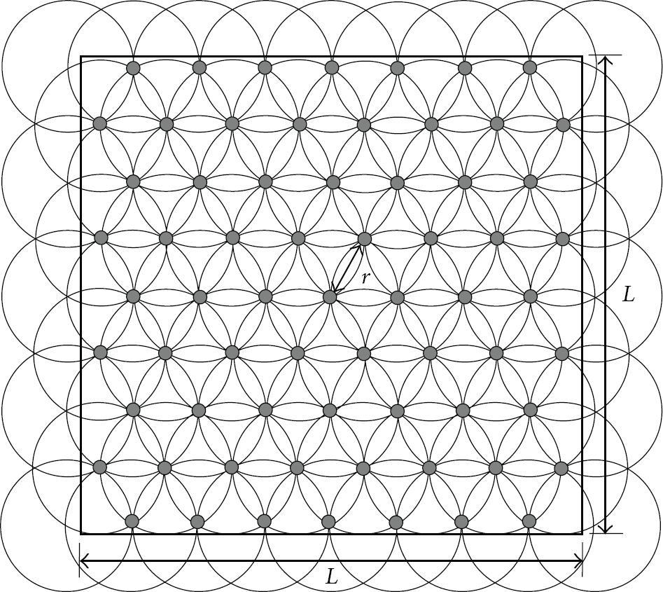
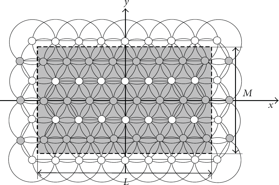
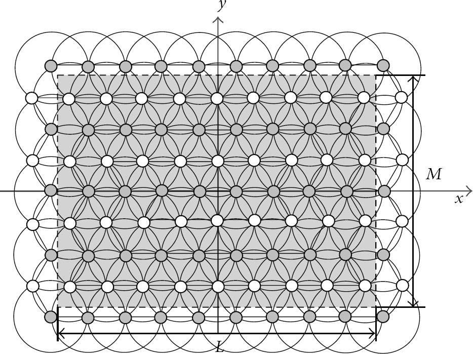
In order to show the moving track of the mobile beacon node in detail, we expand the triple coverage model to a more general case as shown in Figure 3.

Figure 3

Clockwise spiral-like moving path.

The gray rectangular area in Figure 3 is assumed as the sensing region whose length and width are defined as L and M, respectively, and L is no small than M in this case. Then, if the beacon nodes are deployed at all these gray points, unknown nodes at any position in the network will acquire their location in theory.

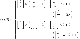
Therefore, the minimum and maximum number of beacon nodes, $N_{\min }$ and $N_{\max }$ , deployed in each line could be calculated as follows:

$$\begin{array}{cc}& N_{\min }=\lceil \frac{L}{r}\rceil +\mathrm{1},\\ N_{\max }=\lceil \frac{L}{r}\rceil +\mathrm{2}.\end{array}$$

(3)

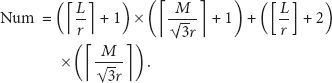
The number of rows about the beacon nodes needs to be deployed in the network is defined as H:

$$\begin{array}{cc}& H=2\lceil \frac{M}{\sqrt{3}r}\rceil +\mathrm{1}.\end{array}$$

(4)

Thus, we could get the total number of the beacon nodes, Num, with the help of

$$\begin{array}{l}\text{Num}=\left(\lceil \frac{L}{r}\rceil +\mathrm{1}\right)\times \left(\lceil \frac{M}{\sqrt{\mathrm{3}}r}\rceil +\mathrm{1}\right)+\left(\left[\frac{L}{r}\right]+\mathrm{2}\right)\\ \hspace{1em}\times \left(\lceil \frac{M}{\sqrt{\mathrm{3}}r}\rceil \right).\end{array}$$

(5)

As a result, if one beacon could move to these gray points one by one, each of unknown nodes anywhere could also calculate out their coordinates.

One of the feasible tracks for the beacon is moving from the first gray point in the upper left corner of the network to the center clockwise along the spiral-like path as shown in Figure 3. It is easy to know that the length of each moving step is r.

3.3. Network Coordinate System

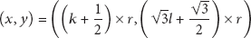
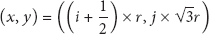
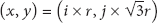
In order to ensure that each of the unknown nodes could acquire the specific running track of the mobile beacon, a type of cartesian coordinates is established as Figure 4 shows and the origin of which is the network center.

Figure 4

The values of $\lceil L/r\rceil$ and $\lceil M/\sqrt{\mathrm{3}}r\rceil$ are all odd numbers.

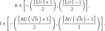
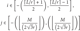
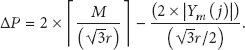
In this paper, the gray points in Figure 3 is called as Broading Points (BPs) because when moving to these points, the beacon node should broadcast their current coordinates to the unknown nodes nearby. Thus, according to the different constraint relationships between L, M, and r, there exist four different cases as follows.

Case 1.

The values of $\lceil L/r\rceil$ and $\lceil M/\sqrt{\mathrm{3}}r\rceil$ are all odd numbers. In this case, there must be a BP at the network center whose coordinate is (0,0), as shown in Figure 4. It is easy to prove that the coordinates of the gray BPs could be calculated by formula (6) and (7) and the white BPs could acquire their position by formulas (8) and (9). The values of i,j, k, and l are all integers:

$$\begin{array}{cc}& \left(x,y\right)=\left(i\times r,j\times \sqrt{\mathrm{3}}r\right)\end{array}$$

(6)

as well as

$$\begin{array}{cc}& i\in \left[-\left(\frac{\lceil L/r\rceil +\mathrm{1}}{\mathrm{2}}\right),\left(\frac{\lceil L/r\rceil +\mathrm{1}}{\mathrm{2}}\right)\right],\\ j\in \left[-\left(\lfloor \frac{M}{\left(\mathrm{2}\sqrt{\mathrm{3}}r\right)}\rfloor \right),\left(\lfloor \frac{M}{\left(\mathrm{2}\sqrt{\mathrm{3}}r\right)}\rfloor \right)\right]\end{array}$$

(7)

or

$$\begin{array}{cc}& \left(x,y\right)=\left(\left(k+\frac{\mathrm{1}}{\mathrm{2}}\right)\times r,\left(\sqrt{\mathrm{3}}l+\frac{\sqrt{\mathrm{3}}}{\mathrm{2}}\right)\times r\right)\end{array}$$

(8)

as well as

$$\begin{array}{cc}& k\in \left[-\left(\frac{\lceil L/r\rceil +\mathrm{1}}{\mathrm{2}}\right),\left(\frac{\lceil L/r\rceil -\mathrm{1}}{\mathrm{2}}\right)\right],\\ l\in \left[-\left(\frac{\lceil M/\left(\sqrt{\mathrm{3}}r\right)+\mathrm{1}\rceil }{\mathrm{2}}\right),\left(\frac{\lceil M/\left(\sqrt{\mathrm{3}}r\right)-\mathrm{1}\rceil }{\mathrm{2}}\right)\right].\end{array}$$

(9)

Case 2.

$\lceil L/r\rceil$ is an even number while $\lceil M/\sqrt{\mathrm{3}}r\rceil$ is an odd one. There is no BP at the network center in this case as shown in Figure 5. Similar to Case 1, the coordinates of the grey BPs in Figure 5 could be calculated by formulas (10) and (11) and the white BPs could acquire their position by formulas by (12) and (13) as follows:

$$\begin{array}{cc}& \left(x,y\right)=\left(\left(i+\frac{\mathrm{1}}{\mathrm{2}}\right)\times r,j\times \sqrt{\mathrm{3}}r\right)\end{array}$$

(10)

while

$$\begin{array}{cc}& i\in \left[-\left(\frac{\lceil L/r\rceil +\mathrm{1}}{\mathrm{2}}\right),\frac{\lceil L/r\rceil }{\mathrm{2}}\right],\\ j\in \left[-\left(\lfloor \frac{M}{\left(\mathrm{2}\sqrt{\mathrm{3}}r\right)}\rfloor \right),\left(\lfloor \frac{M}{\left(\mathrm{2}\sqrt{\mathrm{3}}r\right)}\rfloor \right)\right]\end{array}$$

(11)

or

$$\begin{array}{cc}& \left(x,y\right)=\left(k\times r,\left(\sqrt{\mathrm{3}}l+\frac{\sqrt{\mathrm{3}}}{\mathrm{2}}\right)\times r\right)\end{array}$$

(12)

while

$$\begin{array}{cc}& k\in \left[-\left(\frac{\lceil L/r\rceil }{\mathrm{2}}\right),\left(\frac{\lceil L/r\rceil }{\mathrm{2}}\right)\right],\\ l\in \left[-\left(\frac{\lceil M/\left(\sqrt{\mathrm{3}}r\right)+\mathrm{1}\rceil }{\mathrm{2}}\right),\left(\frac{\lceil M/\left(\sqrt{\mathrm{3}}r\right)-\mathrm{1}\rceil }{\mathrm{2}}\right)\right].\end{array}$$

(13)

Figure 5

$\lceil L/r\rceil$ is an even number and $\lceil M/\sqrt{\mathrm{3}}r\rceil$ is an odd number.

Case 3.

$\lceil L/r\rceil$ is an odd number while $\lceil M/\sqrt{\mathrm{3}}r\rceil$ is an even one. There is also no BP at the network center as shown in Figure 6 and the coordinates of the grey and white BPs could then be calculated by, respectively,

$$\begin{array}{cc}& \left(x,y\right)=\left(\left(i+\frac{\mathrm{1}}{\mathrm{2}}\right)\times r,j\times \sqrt{\mathrm{3}}r\right)\end{array}$$

(14)

as well as

$$\begin{array}{cc}& i\in \left[-\left(\frac{\lceil L/r\rceil +\mathrm{1}}{\mathrm{2}}\right),\frac{\lceil L/r\rceil -\mathrm{1}}{\mathrm{2}}\right],\\ j\in \left[-\left(\lfloor \frac{M}{\left(\mathrm{2}\sqrt{\mathrm{3}}r\right)}\rfloor \right),\left(\lfloor \frac{M}{\left(\mathrm{2}\sqrt{\mathrm{3}}r\right)}\rfloor \right)\right]\end{array}$$

(15)

or

$$\begin{array}{cc}& \left(x,y\right)=\left(k\times r,\left(\sqrt{\mathrm{3}}l+\frac{\sqrt{\mathrm{3}}}{\mathrm{2}}\right)\times r\right)\end{array}$$

(16)

as well as

$$\begin{array}{cc}& k\in \left[-\left(\frac{\lceil L/r\rceil +\mathrm{1}}{\mathrm{2}}\right),\left(\frac{\lceil L/r\rceil +\mathrm{1}}{\mathrm{2}}\right)\right],\\ l\in \left[-\left(\frac{\lceil M/\left(\sqrt{\mathrm{3}}r\right)\rceil }{\mathrm{2}}\right),\left(\frac{\lceil M/\left(\sqrt{\mathrm{3}}r\right)\rceil }{\mathrm{2}}\right)\right].\end{array}$$

(17)

Figure 6

$\lceil L/r\rceil$ is an odd number and $\lceil M/\sqrt{\mathrm{3}}r\rceil$ is an even number.

Case 4.

The values of $\lceil L/r\rceil$ and $\lceil M/\sqrt{\mathrm{3}}r\rceil$ are all even numbers. Similar to Case 1, there must be a BP at the network center in this case (Figure 7). So the grey BPs could be calculated by formulas (18) and (19) and the white BPs could acquire their position by formulas (20) and (21):

$$\begin{array}{cc}& \left(x,y\right)=\left(i\times r,j\times \sqrt{\mathrm{3}}r\right)\end{array}$$

(18)

while

$$\begin{array}{cc}& i\in \left[-\left(\frac{\lceil L/r\rceil }{\mathrm{2}}\right),\left(\frac{\lceil L/r\rceil }{\mathrm{2}}\right)\right],\\ j\in \left[-\frac{\lceil M/\left(\sqrt{\mathrm{3}}r\right)\rceil }{\mathrm{2}},\frac{\lceil M/\left(\sqrt{\mathrm{3}}r\right)\rceil }{\mathrm{2}}\right]\end{array}$$

(19)

or

$$\begin{array}{cc}& \left(x,y\right)=\left(\left(k+\frac{\mathrm{1}}{\mathrm{2}}\right)\times r,\left(\sqrt{\mathrm{3}}l+\frac{\sqrt{\mathrm{3}}}{\mathrm{2}}\right)\times r\right)\end{array}$$

(20)

while

$$\begin{array}{cc}& k\in \left[-\left(\frac{\lceil L/r\rceil }{\mathrm{2}}+\mathrm{1}\right),\left(\frac{\lceil L/r\rceil }{\mathrm{2}}\right)\right],\\ l\in \left[-\left(\frac{\lceil M/\left(\sqrt{\mathrm{3}}r\right)\rceil }{\mathrm{2}}\right),\left(\frac{\lceil M/\left(\sqrt{\mathrm{3}}r\right)\rceil }{\mathrm{2}}\right)\right].\end{array}$$

(21)

Figure 7

The values of $\lceil L/r\rceil$ and $\lceil M/\sqrt{\mathrm{3}}r\rceil$ are all even numbers.

3.4. Node Localization Based on Mobile Beacon

3.4.1. Moving and Broadcasting Strategy

The behavior of the beacon for localization could be described as follows.

Step 1.

The beacon moves from the left corner to the network center clockwise along with the spiral-like path. Its step size and moving speed are r and v, respectively.

Step 2.

The beacon stays at each BP for a period of time, defined as t. During this period, it broadcasts its coordinate continuously. The unknown nodes in the beacon's communicate range could receive the data packet when they are in listening mode.

Step 3.

The localization algorithm terminates when the beacon moves to the end of the spiral-like path.

3.4.2. Localization Process and Sleeping Scheduling Strategy for Unknown Nodes

According to the track of the mobile beacon, it is easy to see that when one of the unknown nodes received the coordinate information about the mobile beacon for the first time, the following situations may occur.

Case 1.

This unknown node could no longer receive any information from the beacon when it moves to the next BP and broadcasts its coordinate at that point. For example, the unknown node $n_1$ in Figure 8 could not communicate with the beacon when it moves from $S_1$ to $S_2$ . Furthermore, the next time $n_2$ receives the coordinate information again is the moment when the beacon just arrives at $S_4$ .

Figure 8

Localization process for unknown nodes.

Case 2.

The unknown node is still in the beacon's broadcasting range when it moves to the next BP. As shown in Figure 8, $n_2$ could receive the broadcasting information no matter the beacon is at $S_1$ or $S_2$ . However, in this case, it could not receive the beacon's coordinate again when the beacon moves to $S_3$ .

Case 3.

After receiving the coordinate information for the first time, the unknown node could continuously communicate with the mobile beacon when the beacon moves to the next two BPs. As shown in Figure 8, $n_3$ could successively receive the coordinate information of the beacon which stays in $S_5$ , $S_6$ , and $S_7$ .

In addition, it is easy to know that, after communicating with the beacon for the first time, any one of the unknown nodes would at least receive the beacon's real-time coordinate information again when it rotates a circle according to the spiral-like moving path. The length of the time interval between these two information exchanges depends on the moving speed and step size of the beacon. Hence, the sleep scheduling algorithm for localization is described as follows.

Step 1.

The unknown nodes in the network are all in listening mode at the beginning of the localization.

Step 2.

When any one of the unknown nodes, named as $n_i$ for simplicity, receives the data packets broadcasted by the mobile beacon for the first time, it will further analyse the beacon's coordinate info, $(X_m(j),Y_m(j))$ , as follows.

If $|Y_m(j)/X_m(j)|\ge |M/L|$ , we define an auxiliary parameter $\mathrm{\Delta }P$ , as follows:

$$\begin{array}{cc}& \mathrm{\Delta }P=\mathrm{2}\times \lceil \frac{M}{\left(\sqrt{\mathrm{3}}r\right)}\rceil -\frac{\left(\mathrm{2}\times \left|Y_m\left(j\right)\right|\right)}{\left(\sqrt{\mathrm{3}}r/\mathrm{2}\right)}.\end{array}$$

(22)

Furthermore, PTIE is defined as a consecutive period of time for information exchange between the beacon and $n_i$ . Therefore, the length of PTIE is from the time when $n_i$ just acquires the real-time coordinate of the beacon to the time when the beacon leaves form the last BP in $n_i$ 's communication range. Then the length of time interval between two PTIEs could be approximatively calculated by

$$\begin{array}{l}\mathrm{\Delta }T\left(S_i\right)=\left(\frac{r}{v}+t\right)\times \{\mathrm{2}\times [f\left(\mathrm{2}\lceil \frac{M}{\left(\sqrt{\mathrm{3}}r\right)}\rceil -\mathrm{\Delta }P-\mathrm{1}\right)\\ \hspace{1em}\hspace{1em}\hspace{1em}\hspace{1em}\hspace{1em}\hspace{1em}\hspace{1em}\hspace{1em}\hspace{1em}\hspace{1em}\hspace{1em}+f\left(\lceil \frac{L}{r}\rceil -\mathrm{\Delta }P-\mathrm{1}\right)\phantom{\mathrm{2}[f\left(\mathrm{2}\lceil \frac{M}{\left(\sqrt{\mathrm{3}}r\right)}\rceil -\mathrm{\Delta }P-\mathrm{1}\right)}]-\mathrm{2}\}.\end{array}$$

(23)

In which, the value of $f(x)$ could be defined as follows:

$$\begin{array}{cc}& f\left(x\right)=\{\begin{array}{cc}x\hfill & \text{if}\hspace{0.17em}\hspace{0.17em}x\ge \mathrm{0},\hfill \\ \mathrm{0}\hfill & \text{if}\hspace{0.17em}\hspace{0.17em}x<\mathrm{0}.\hfill \end{array}\end{array}$$

(24)

If $|Y_m(j)/X_m(j)|<|M/L|$ , the length of time interval between two PTIEs, $\mathrm{\Delta }T(S_i)$ , could then be expressed as formula (26) in which the value of $\mathrm{\Delta }Q$ could be calculated by

$$\begin{array}{ll}& \mathrm{\Delta }Q=\lceil \frac{L}{r}\rceil -\mathrm{2}\times \left(\frac{\left|X_m\left(j\right)\right|}{r}\right)\end{array}$$

(25)

$$\begin{array}{l}\mathrm{\Delta }T\left(S_i\right)=\left(\frac{r}{v}+t\right)\times \{\phantom{f\left(\mathrm{2}\lceil \frac{M}{\left(\sqrt{\mathrm{3}}r\right)}\rceil -\mathrm{\Delta }P-\mathrm{1}\right)}\mathrm{2}[f\times \left(\mathrm{2}\lceil \frac{M}{\left(\sqrt{\mathrm{3}}r\right)}\rceil -\mathrm{\Delta }Q-\mathrm{1}\right)\\ \hspace{1em}\hspace{1em}\hspace{1em}\hspace{1em}\hspace{1em}\hspace{1em}\hspace{1em}\hspace{1em}\hspace{1em}\hspace{1em}+f\left(\mathrm{2}\left(\frac{\left|X_m\left(j\right)\right|}{r}\right)-\mathrm{1}\right)\phantom{f\left(\mathrm{2}\lceil \frac{M}{\left(\sqrt{\mathrm{3}}r\right)}\rceil -\mathrm{\Delta }P-\mathrm{1}\right)}]-\mathrm{2}\}.\end{array}$$

(26)

Step 3.

In our model, it is easy to know that the unknown nodes could not receive sufficient coordinate information of the beacon for localization in one PTIE. As shown in Figure 8, the unknown node $n_2$ could only acquire two different coordinates when the beacon moves to $S_1$ and $S_2$ in the first PTIE. Therefore, to accomplish localization, any one of the unknown nodes needs to communicate with the beacon in two PTIEs. Consequently, if they could stay in sleeping mode during $\mathrm{\Delta }T(S_i)$ , the time interval between the two PTIEs, the energy consumption in localization might be reduced.

However, the energy consumption during node's mode switching could not be ignored. Thus, the following formula is proposed:

$$\begin{array}{cc}& \mathrm{\Delta }T\left(S_i\right)\times P_{\text{sleep}}+\mathrm{2}\times E_{\text{switch}}<\mathrm{\Delta }T\left(S_i\right)\times P_{\text{listen}}.\end{array}$$

(27)

It would save energy when the unknown node be is the sleeping mode during $\mathrm{\Delta }T(S_i)$ if and only if formula (27) holds up. $P_{\text{sleep}}$ and $P_{\text{listen}}$ are defined as the power consumption of the unknown node in sleeping and listening mode, respectively, and $E_{\text{switch}}$ is the energy consumption in mode switching. Thus, the energy consumption reduced for an unknown node in its localization process could be calculated by

$$\begin{array}{cc}& \mathrm{\Delta }E=\mathrm{\Delta }T\left(S_i\right)\times \left(P_{\text{listen}}-P_{\text{sleep}}\right)+\mathrm{2}\times E_{\text{switch}}.\end{array}$$

(28)

Step 4.

After acquiring three or more coordinates in two PTIEs, the unknown node could calculate out its location with the help of the LQI based localization method mentioned in Section 3.4.3.

3.4.3. Localization Based on the Value of LQI

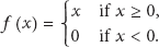
As we know, the free-space model, two-ray ground reflection model, and the shadowing model are the typical signal propagation models in Wireless Sensor Networks. Without losing of generality, we use the free-space propagation model [23] to calculate the distance between the beacon and unknown node in

$$\begin{array}{cc}& L\left(\text{dB}\right)=PL\left(d_{\mathrm{0}}\right)+\mathrm{10}\times \eta \times \text{lg}\left[\frac{d\left(S_i,S_j\right)}{d_{\mathrm{0}}}\right]+X_{\sigma },\\ \text{RSSI}\left(S_i,S_j\right)=P_T-L\left(\text{dB}\right).\end{array}$$

(29)

$S_i$ and $S_j$ are the sender and receiver, respectively, and the distance between them is $d(S_i,S_j)$ . $\text{RSSI}\hspace{0.17em}(S_i,S_j)$ is the signal strength received by $S_j$ and η denotes the path loss factor whose default value is 4. $P_T$ and $PL\hspace{0.17em}(d_{\mathrm{0}})$ are regarded as the transmission power and the reference received power, respectively, and the values of them are −5 dBm and 55 dB [24]. $X_{\sigma }$ is defined as a random variable and its mean and variance are 0 and 5.

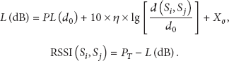
Therefore,

$$\begin{array}{cc}& \text{RSSI}\left(S_i,S_j\right)=P_T-PL\left(d_{\mathrm{0}}\right)-\mathrm{10}\times \eta \times \text{lg}\left(\frac{d}{d_{\mathrm{0}}}\right)+X_{\sigma }.\end{array}$$

(30)

In most range-based localization algorithm, the distance between the sender and receiver could be calculated with the help of the Received Signal Strength Indication (RSSI). However, the value of RSSI could not be directly obtained from the data packet and we use the link quality indicator (LQI for short) [25] for distance computation. The value of LQI varies from 0 to 255 with high accuracy and it could be obtained from the MAC layer directly. The relationship between RSSI and LQI is shown in formula (31) [26] and the values of α and β are affected by the environment. Thus, the unknown node would finish its localization with the help of a series of LQIs that it acquires

$$\begin{array}{cc}& \text{LQI}\left(S_i,S_j\right)=\alpha +\beta \times \text{RSSI}\left(S_i,S_j\right).\end{array}$$

(31)

4. Simulation Results

To testify the effect of localization with the mobile beacon, the simulation is operated under Omnet++3.2 and Matlab7.0. We compare our SMP method to the static localization method by RSSI and maximum likelihood estimation as well as the DV-HOP method. Moreover, we also simulate the localization process about the virtual force based method with the help of a TSP based beacon moving model mentioned in [19].

4.1. Localization Error

Mean values of error about these four types of localization methods are shown in Figure 9 and values of the parameters during this experiment are set in Table 1. It can be seen from the figure that the SMP localization method has the best performance. The mean value of error about it is smaller than 12% and is relatively steady. This is because the mobile beacon moves along the spiral-like path expanded by the triple coverage model which ensures that all of the unknown nodes could acquire three or four beacon nodes’ location-specific information nearby and could calculate out their coordinates accurately. Moreover, during the localization process, the mobile beacon broadcasts its coordinate if and only if it arrives at one of the BPs and the unknown nodes only need to be in listening state which avoids the interference of signals. While In TSP based moving model, beacon affected by the virtual repulsive force could hardly move to the network boundary which reduces the accuracy of localization [19].

Table 1

Values of parameters.

Parameter	Symbol	Value	Unit
Network size	L × M	200 × 100	M2
Communication radius of node	r	20	M
Number of beacons in static localization method	$N(B)$	80
Length of time for the mobile beacon staying at each BP	t	10	S

Figure 9

Mean values of error.

The standard deviation of these localization algorithms is shown in Figure 10. In SMP method, most of the unknown nodes in the network could receive relatively accurate value of each LQI because the beacon could move along the spiral-like path and broadcast its coordinate at each BP. Therefore, the localization error of each unknown node is close to each other. Moreover, it is easy to know that the accuracy of localization in SMP has nothing to do with the number of the unknown nodes as well as their distribution, which keeps the standard deviation stable. However, in TSP based moving mode, the localization error of the unknown nodes near the boundary of the network is larger which increase the standard deviation.

Figure 10

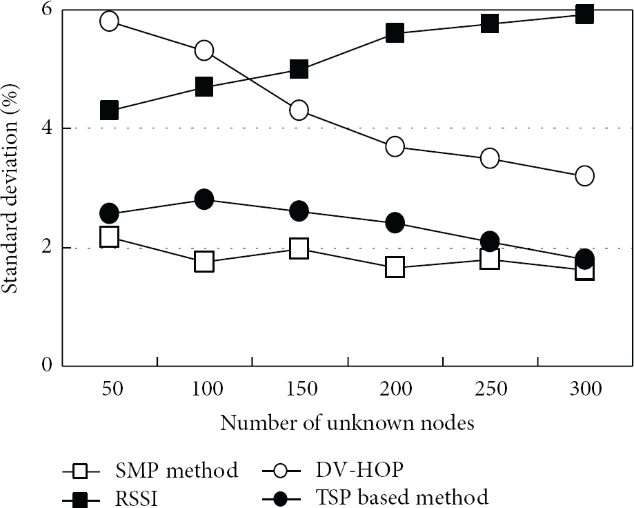
Standard deviation about localization.

4.2. Success Rate about Localization

Figures 11 and 12 show the success rate about localization of the four methods under different network sizes. The success rate is defined as the ratio about the number of nodes whose localization error is smaller than the threshold (set as 30%) and the total number of the unknown nodes in the network. As we see, the SMP localization method also has the best performance regardless of the network size as well as the number of the unknown nodes. This is because the BPs are uniformly distributed in the network in our model, so each of the unknown nodes could receive sufficient coordinates to enhance the success rate.

Figure 11

Success rate about localization (network size is 200 M × 100 M).

Figure 12

Success rate about localization (network size is 300 M × 200 M).

In particular, when the parameter t is larger, the beacon will stay at each BP for a long time which ensures that the unknown nodes nearby could receive the accurate coordinate information of the beacon that will further increase the success rate about localization.

4.3. Percentage of Nodes in Sleeping Mode

Table 2 shows the percentage of unknown nodes in sleeping mode during the time interval between the two PTIEs. In this experiment, $v=10\hspace{0.17em}\text{m/s}$ , $t=5\hspace{0.17em}\text{s}$ , and $r=20\hspace{0.17em}\text{m}$ . It is easy to see that this percentage is stable and high when the network size is fixed. Whether or not the unknown node could be in sleeping mode is related to the value of $\mathrm{\Delta }T(S_i)$ , which is subjected to the value of L, M, v, t, and r, according to formulas (27) and (28). While in our model, the above parameters are all fixed, so the values of the percentage of unknown nodes in sleeping mode keep stable.

Table 2

Percentage of unknown nodes in sleeping mode.

Network size $L\times M=$   200 × 100, Unit: M
$N_l$	50	100	150	200	250	300
$N_s$	37	72	111	159	189	239
K	74%	72%	74%	79.5%	75.6%	79.7%
Network size $L\times M=$   300 × 200, Unit: M
$N_l$	50	100	150	200	250	300
$N_s$	41	81	133	169	220	258
K	82%	81%	88.7%	84.5%	88%	86%

( $N_l$ : number of the unknown nodes; $N_s$ : number of the sleeping nodes; K: percentage).

On the other hand, with the expansion of the network, the value of $\mathrm{\Delta }T(S_i)$ will increase. And because $P_{\text{sleep}}$ is far less than $P_{\text{listen}}$ , there must be more nodes in sleeping mode. Thus, the percentage of unknown nodes in sleeping mode will increase when the network size is larger.

4.4. Energy Consumption in Localization

Figures 13 and 14 show the energy consumption of the network during the localization process. For the sake of simplicity, we ignore the mobile beacon's energy consumption in SMP method. As we see, in SMP, most of the unknown nodes could go into sleeping mode most of the time during the localization process and the unknown nodes do not need to send any message to the beacon which greatly reduces the energy consumption in localization.

Figure 13

Energy consumption in localization (network size is 200 M × 100 M).

Figure 14

Energy consumption in localization (network size is 300 M × 200 M).

Although the triple coverage model is also used in the TSP based beacon moving model, this localization method could only apply to the network with a circular shape and the redundancy of coverage is also high. Furthermore, the number of BPs of this algorithm is more than the SMP method which leads to high energy consumption.

From Figures 13 and 14, it is also known that the average energy consumption in SMP is unrelated to the number of the unknown nodes, because the distributed computing method is used in SMP and nodes do not need to communicate with its neighbors during the localization process.

5. Conclusion

A type of energy efficient localization method based on mobile beacon is proposed in this paper. Each of the unknown nodes could not only acquire sufficient information of the beacon, but also go into sleeping mode to save energy. Simulation results show that the SMP method increases the accuracy of localization for Wireless Sensor Networks and reduces energy consumption of the unknown nodes.