
Abstract
Three active front-steering (AFS) controllers were developed to enhance the lateral stability of a vehicle. They were designed using proportional-integral-derivative (PID), fuzzy-logic, and sliding-mode control methods. The controllers were compared under several driving and road conditions with and without the application of braking force. A 14-degree-of-freedom vehicle model, a sliding-mode antilock brake system (ABS) controller, and a driver model were also employed to test the controllers. The results show that the three AFS controllers allowed the yaw rate to follow the reference yaw rate very well, and consequently the lateral stability improved. On a split-μ road, the controllers forced the vehicle to proceed straight ahead. The results also verify that the driver model can sufficiently control the vehicle to allow it to follow a desired path.
1. Introduction
Active front steering (AFS) provides an electronically controlled superposition of an angle on the steering wheel angle. However, a permanent mechanical connection between the steering wheel and the road wheels remains. This additional degree of freedom enables a continuous and driving-situation-dependent adaptation of the steering characteristics. Features such as steering comfort, effort, and steering dynamics are optimized, and stabilizing steering interventions can be performed [1].
Figure 1 shows the AFS principle: the driver controls the course of the vehicle via the steering wheel. The resulting steering wheel angle is denoted by δ d . The AFS actuates an additional angle using its electric motor. Both angles result in a pinion angle δ p at the steering rack. The resulting road-wheel angle can then be calculated via the pinion angle, as well as a static nonlinearity that accounts for the relationship between the pinion angle and rack displacement for the steering geometry [2].
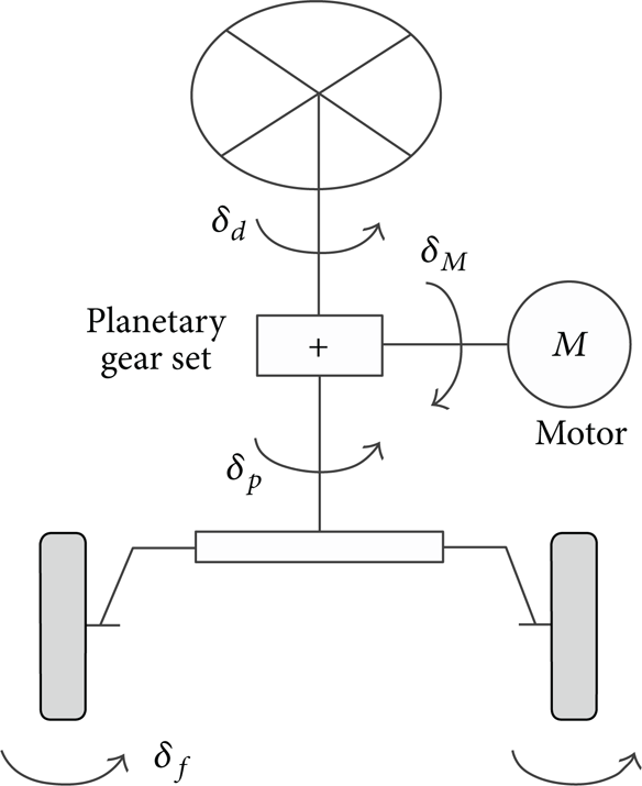
AFS system.
AFS was developed and commercialized by ZF Lenksysteme and BMW AG. Many AFS-related studies were reported following this event. Oraby developed an AFS control strategy that was based on optimal control theory using the linear quadratic regulator (LQR) technique [3]. Klier and Reinelt designed a mathematical model of an AFS system including eight rigid bodies, 46 constraint relations, and a synchronous motor [2]. Zhang et al. developed a quantitative feedback theory (QFT) and evaluated the control system under various emergency maneuvers and road conditions [4]. Ahmed et al. developed an AFIS (active front independent steering) system [5]. It controls the steer angle of front inner and outer wheels independently to equalize the tire workload of two wheels. Namuduri et al. proposed a control methodology developed to make a low-cost brushless permanent magnet motor drive (BLDC) suitable for the AFS application [6]. They designed a simulation model and used a conventional PID controller to achieve smooth operation of the AFS actuator and to prevent unwanted vibration at the steering wheel. However, these studies are not sufficient if we consider the importance of AFS on vehicle stability. Although active front-wheel steering systems are being studied extensively, the development of control strategies has largely been the focus. The performance of the AFS has been neglected.
Additionally, most AFS-related studies developed the AFS as a part of an integrated chassis control system (unified chassis control system (UCC)) and not as a single stand-alone system. Usually, AFS is integrated with an active brake control system [7–9], active rear wheel control system [10], or active suspension control system [11, 12]. Thus, those studies have not focused on the development of AFS. This may be due to poor AFS performance. AFS can control only one control variable at a time, such as yaw rate, but an integrated control system can modify two or more control variables simultaneously, such as yaw rate and body slip angle or yaw rate and ride comfort.
In this study, we designed AFS controllers to enhance vehicle safety, stability, and steerability. In addition, we identified the optimal control method to enhance AFS performance. Three different AFS control algorithms were developed and tested, that is, proportional-integral-derivative (PID) control, fuzzy-logic control (FLC), and sliding-mode control (SMC). To accomplish this task, a 14-degree-of-freedom (DOF) vehicle, a sliding-mode antilock brake system (ABS) controller, and a driver model were used. A two-degree-of-freedom vehicle model was also employed to design the SMC.
2. Vehicle and Driver Models
2.1. Fourteen-Degree-of-Freedom Vehicle Model
A nonlinear vehicle dynamics model was used for the simulations. This model had 14 DOF that included the three in-plane motions of the vehicle (X, Y, γ), the roll motion (ϕ), and the rotational dynamics of each of the four wheels (ω i ). Figure 2 shows the vehicle model with the coordinate system, degrees of freedom, and external forces. A list of notations is provided in the Notation Section. The equations of motion for the model are as follows [13–15].

14-degree-of-freedom vehicle model.
Longitudinal motion:

Lateral motion:

Yaw motion:

Roll motion:

Pitch motion:

Wheel motion:

Sprung mass motion:

Unsprung mass motion:
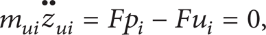
where

In these equations, the subscripts i are 1, 2, 3, and 4 for the left front, right front, left rear, and right rear wheels, respectively.
2.2. Two-Degree-of-Freedom Vehicle Model
A 2 DOF vehicle model was also developed for the sliding-mode AFS controller. The state space representation of the 2-DOF vehicle model is given as [3, 7]

where the state vector x, the input vector u, the system matrix A, and the input matrix B are defined by
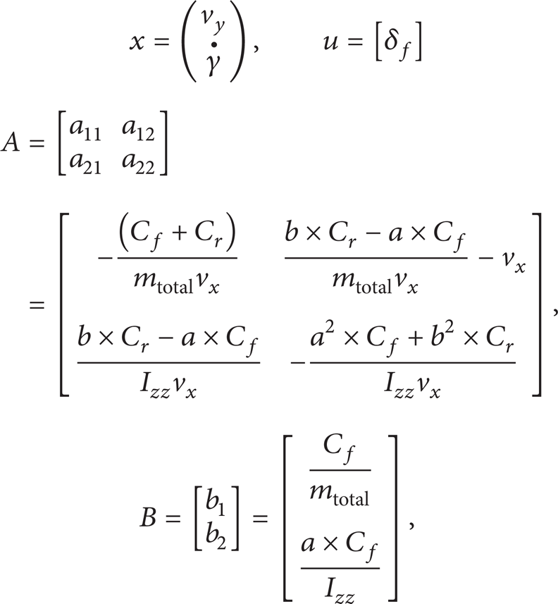
where δ f is the front-wheel steering angle. C f and C r are the front and rear axle cornering stiffnesses and are 105850.0 N/rad and 79030.0 N/rad, respectively.
2.3. Driver Model
A driver model is required to direct a vehicle to follow a desired path. However, it is difficult to design a driver model because the behavior of a driver depends on physical and psychological factors, as well as the demands of the driving situation [14, 16]. To date, descriptions of driver behavior have not been sufficiently realistic.
In this paper, we assumed that the steering angle is a function of the estimated lateral offset of the vehicle center of gravity (CG) from the desired path (∊) at the look-ahead distance (L) and the yaw angle (γ) of the CG (Figure 3). This assumption can be represented mathematically as

where τ s is the time delay of the driver's response (approximately 0.1 to 0.3 seconds) and a1, a2, and a3 are constants [16].

Strategy of the driver model [14].
3. Controller Designs
Four controllers were used in this study. Three were for AFS systems and one was for an ABS system. The ABS controller was designed to implement the desired slip by controlling the brake pressure. The desired slip was defined as 0.15, regardless of the road conditions. Previous studies by the author fully describe the ABS controller [13–15].
The three controllers for the AFS system controlled the front steering angle to allow the yaw rate to track the reference yaw rate. The reference yaw rate is determined by [15]

where

To avoid large lateral acceleration that exceeds the tire cornering capability, the yaw rate was constrained as [17]

3.1. AFS Sliding-Mode Controller
In the case of AFS, the yaw motion of the vehicle can be expressed as the following single-input single-output (SISO) affine system, that is, a nonlinear system with the right-hand side of the equation of motion expressed as a linear function of the control input [18]:
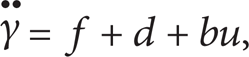
where
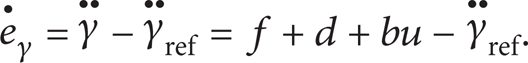
For the yaw rate tracking task, the difference between the actual and reference yaw rate defines the tracking error:

And derivative of the tracking error is
The sliding surface is then selected as

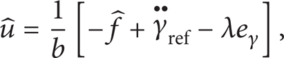
where λ is a strictly positive constant. If there are no dynamic uncertainties or disturbances affecting the system, the equivalent control input can be obtained as

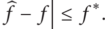
The best approximation
if we define

where η is a strictly positive constant. Since
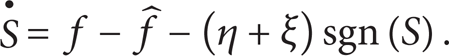
If we define ξ as
then (24) satisfies the sliding condition

Therefore, the control input u is obtained from (22), (23), and (23) as follows:

Substituting the second-state equation of (10) into (27) gives

The chattering problem caused by the control discontinuity of the sgn (S) function can be eliminated by using a thin boundary layer of thickness Φ neighboring the switching surface. Hence, sgn (S) of (28) can be replaced by the function sat (S/Φ). The continuous approximation of the control law in (28) can be expressed as

The control law of (29) can be directly applied to steering-by-wire systems. In the case of steering correction control systems, the control input in (29) is the steering angle at the front wheels; hence, the corrective steering angle is the difference between the AFS controller output and the driver steering inputs:
3.2. AFS PID Controller
A PID controller is a generic control-loop feedback controller widely used in theoretical and practical control systems. The error, which is the difference between the desired and measured variables, is an input to the PID controller. The desired variable is the reference yaw rate, and the measured variable is the yaw rate. The controller attempts to minimize the error by adjusting the control output which is the steering angle of the wheel. The front-wheel steering angle, δ f , is calculated by the next PID controller

where K P , K I , and K D are the proportional, integral, and derivative gains, respectively, and τ is the variable of integration. Equation (31) can be discretized as

The gains are tuned and determined by Ziegler-Nichols method [19].
3.3. AFS Fuzzy Controller
A fuzzy controller design consists of (1) the definition of the input-output fuzzy variables, (2) decision-making procedures related to the fuzzy control rules, (3) fuzzy inference logic, and (4) defuzzification [20, 21].
An AFS fuzzy controller consists of two input and one output variables. The inputs are the yaw rate error and its derivative. Fuzzification made the measured controller inputs dimensionally compatible with the condition of the knowledge-based rules using suitable linguistic variables [21]. The yaw rate error input variables have seven triangular membership functions with a universe of discourse of [−0.5, 0.5] (Figure 4 (a)). The input error derivative variables have five triangular membership functions with a universe of discourse of [−1, 1] (Figure 4 (b)). The universes of discourse of the inputs are selected based on the ranges of the error and its derivative without the controller.

Membership functions for inputs (a) eγ and (b)
The output of the AFS fuzzy controller is the corrective steering angle of the front wheels (Δδ f ). The output variables are composed of seven triangular membership functions with a universe of discourse of [−0.5, 0.5] (Figure 4 (c)).
The output variable is calculated based on appropriate rules of fuzzy control theory. The rule base used in the system is shown in Table 1, with fuzzy terms derived by modeling the designer's knowledge, experience, and simulation. The fuzzy controller used the Mamdani fuzzy inference system [21], which is characterized by the following fuzzy rule schema:
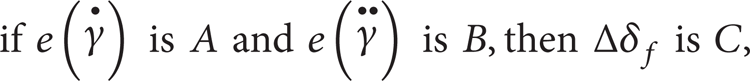
where A, B, and C are fuzzy sets defined on the input and output domains, respectively.
Fuzzy rules for corrective front steer angle.

4. Results and Discussion
The developed controllers were tested in a vehicle running on various road conditions and steering inputs. The performances were validated with and without brake pressure.
4.1. Condition When Brake Pressure Was Applied
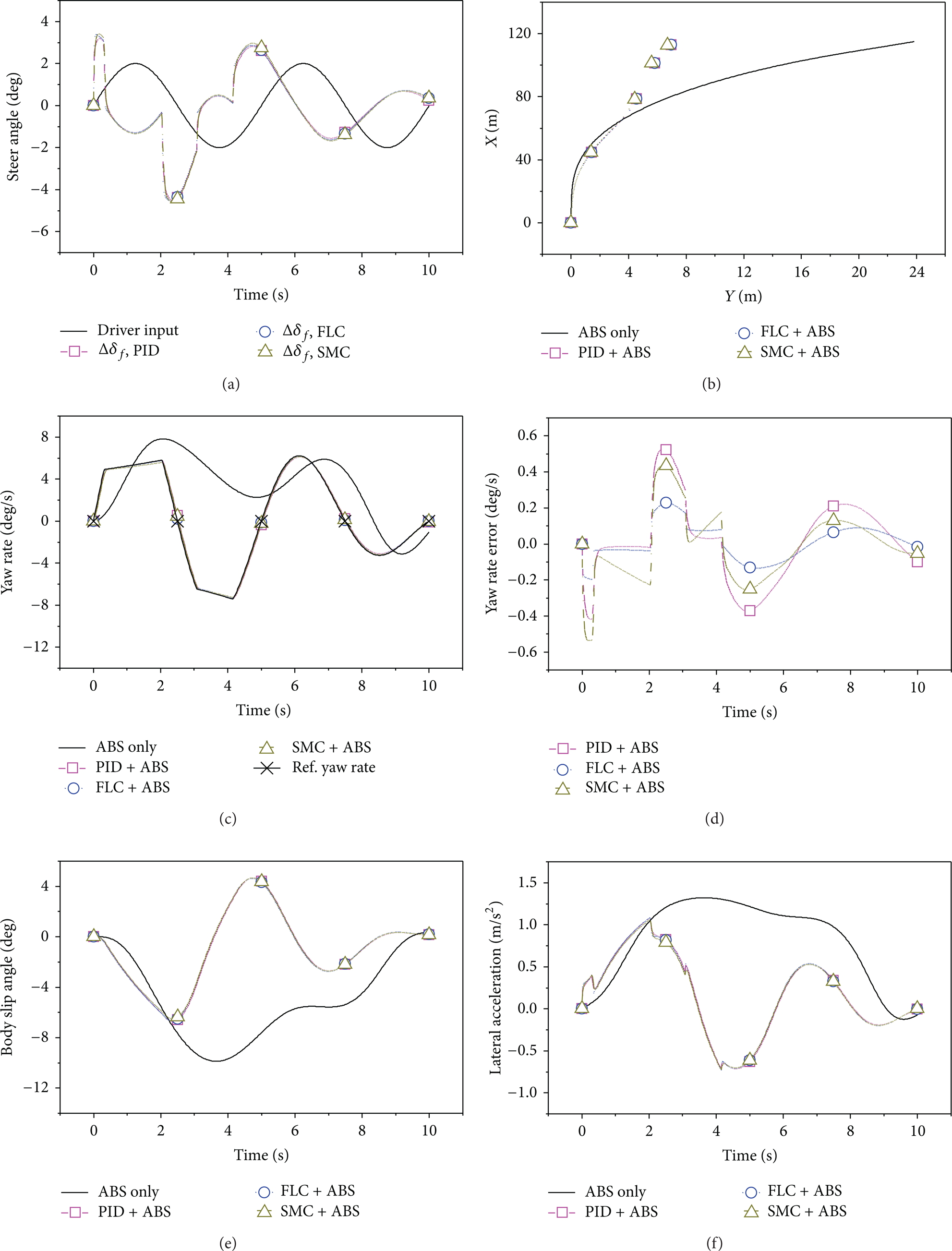
Figure 5 shows the vehicle and controller responses when a sinusoidal steering input was applied. We assumed that the vehicle was running on dry asphalt with an initial velocity of 30 m/s. Full brake pressure was applied at zero seconds; an ABS controller engaged as a result.

Vehicle responses when sinusoidal steering and full braking inputs are applied on dry asphalt.
The steering input by the driver and additional steering input by the controllers are shown in Figure 5 (a). The yaw rates and the reference yaw rate of the PID, FLC, and SMC vehicles are shown in Figure 5 (c). The yaw rates of the three vehicles tracked the reference yaw rate very well, which indicates that the controllers enhanced the stability of the vehicle [11, 13]. The distortion of the yaw rate between about 0.4 and 1.3 s was due to the yaw rate constraint. This constraint can be considered as a disturbance; the results demonstrate that the developed controllers were very robust towards disturbance.
Because the objective of the three controllers is to allow yaw rate to track reference yaw rate, the yaw rates of three controllers will be very similar if they work properly. Similar yaw rates mean that the response of the vehicle is similar. The trajectory (Figure 5 (b)), the body slip angle (Figure 5 (e)), and the lateral acceleration (Figure 5 (f)) were all similar. However, Figure 5 (d) shows that the yaw rate error of the FLC was the smallest.
Figures 5 (e) and 5 (f) depict the body slip angle and the lateral acceleration. The smaller body slip angle due to the controllers demonstrates that the controllability improved, but a smaller lateral acceleration represented a larger turning radius (Figure 5 (b)). Thus, improvement of controllability was weak.
The controllers were also tested on a snow-covered road at an initial velocity of 20 m/s. The ABS also engaged at zero seconds and the responses were compared. Figure 6 shows the steering input and vehicle performances. The yaw rates of the PID-, FLC-, and SMC-controlled vehicles followed the reference yaw rate very well (Figure 6 (c)), even when disturbances were present. Figure 6 (d) also shows that the yaw rate error of the FLC was the smallest among the three controllers.
Vehicle responses when sinusoidal steering and full braking inputs are applied on snow-covered road.
The vehicle trajectory (Figure 6 (b)), yaw rate, and lateral acceleration (Figure 6 (f)) of the three controllers show that steerability was maintained; this was not the case with the ABS-controlled vehicle. That vehicle could not respond to a sinusoidal steering input, as shown in the figures. The larger body slip angle (Figure 6 (e)) also indicates that the steerability was worse.
Figures 7 and 8 show the vehicle responses and trajectories when they ran on a split-μ road and full brake pressure was applied from zero seconds. We assumed that the right side of the CG was dry asphalt and the left side was a snow-covered road. The initial velocity was 30 m/s.

Vehicle responses on split-μ road (dry asphalt and snow-covered road).
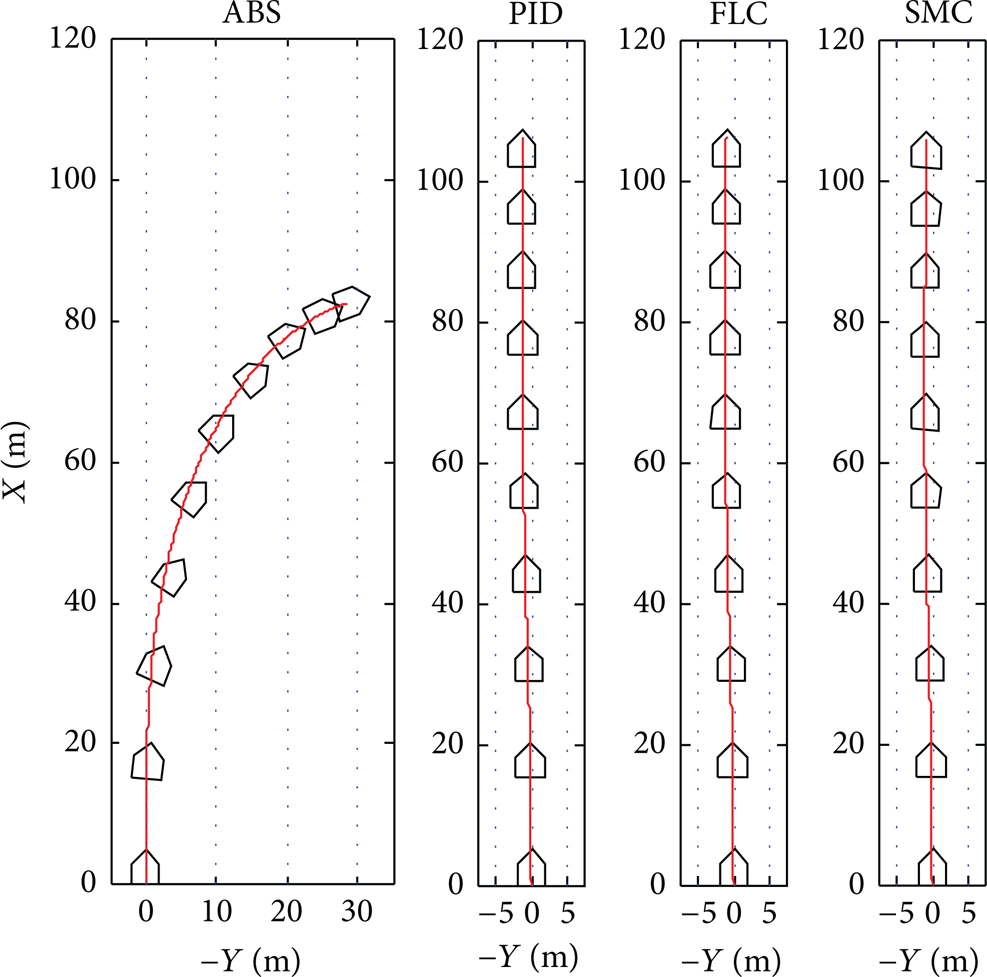
Vehicle trajectory on split-μ road (dry asphalt and snow-covered road).
When a vehicle runs on a split-μ road and braking force is applied, it moves to the side having the higher coefficient of friction because of different tire forces between the left and right sides. Figures 7 (b), 7 (c), and 7 (d) and Figure 8 show the lateral dynamics of the ABS-equipped vehicle even though the steering input was zero. However, when the PID, fuzzy, or sliding-mode controller was applied, the vehicle proceeded almost straight ahead and moved forward. This indicates that the stability and steerability were improved and enhanced.
4.2. Condition When Brake Pressure Was Not Applied
The performance of the AFS was tested when neither braking force nor traction force was applied. Figure 9 (a) shows the vehicle responses to a sinusoidal steering input (Figures 9 (b)–9 (f)) when they ran on wet asphalt. The initial velocity was 25 m/s.
Vehicle responses when sinusoidal steering and no braking inputs are applied on wet asphalt.
The lateral stability of the uncontrolled vehicle worsened as the steering input increased. However, when the PID, FLC, or SMC was adopted, controllability improved and the vehicle responded properly to the steering input, as shown in Figures 9 (b), 9 (c), 9 (e), and 9 (f). The reference yaw rate was also distorted, but the yaw rates of the PID and SMC followed it very well. In case of the FLC, the performance worsened after about 8 seconds. The corrective steering angle fluctuated and the yaw rate was delayed. As a result, the yaw rate error increased (Figure 9 (d)), the lateral acceleration oscillated (Figure 9 (f)), and the trajectory deviated (Figure 9 (b)). Because a braking maneuver was used to tune the fuzzy rule, the FLC had the worst performance between controllers when brake pressure was not applied. Thus, when an AFS controller is designed with an FLC, the fuzzy rule must be fine-tuned.
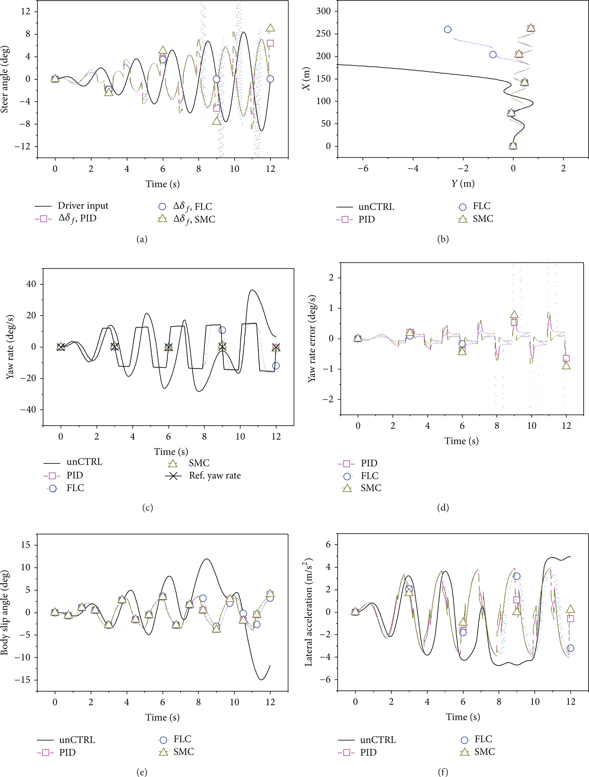
Figure 10 shows the responses of a vehicle that traveled on a snow-covered road and executed a double lane-change. The initial velocity was 15 m/s, and the driver model steered the vehicle. Figure 10 (a) shows the steering inputs for the uncontrolled and PID-controlled conditions, and Figure 10 (b) depicts the FLC-controlled and SMC-controlled conditions. A strongly fluctuating steering input was needed to follow the desired path for the vehicle not equipped with the controllers. It induced an unstable yaw rate and lateral acceleration, as well as a larger body slip angle. However, the AFS controller required similar but less fluctuating steering inputs, and the yaw rate followed the reference yaw rate very well. The AFS-controlled vehicle behaved similarly (Figures 10 (c), 10 (e), and 10 (f)) but the FLC had the largest yaw rate error, although the error had little effect because its maximum value was only about 5% of the yaw rate.

Vehicle responses when a driver model steers and no brake inputs are applied on snow-covered road.
Figure 11 shows the trajectories of the controlled and uncontrolled vehicles. The results show that the vehicle followed the lateral displacement almost perfectly in the presence or absence of an AFS controller. These results also demonstrate that the driver model sufficiently controlled the vehicle to allow it to follow the desired path.

Trajectories of vehicle equipped with PID controller, FLC and SMC.
5. Conclusions
In this study, AFS controllers were developed using PID, FLC, and SMC methods, and their performances were tested under several driving conditions. A fourteen-degree nonlinear vehicle model, a sliding mode ABS controller, and a driver model were used. The conclusions of this study are as follows.
The developed SMC and PID controllers controlled the additional steering angle and enhanced the lateral stability. They had excellent performances because the yaw rates followed the reference yaw rate in every driving condition.
The performance of the FLC was the best among the developed controllers during a braking maneuver. However, it was the worst when brake pressure was not applied. This is because a braking maneuver was used to tune the fuzzy rules.
When a vehicle ran on a split-μ road and brake pressure was applied, the vehicle was directed towards the side with the higher coefficient of friction and the steerability deteriorated. However, the AFS controllers modified the front steering angle, forced the vehicle to proceed almost straight ahead, and increased the vehicle stability.
A driver model was developed and tested on a snow-covered road. It controlled the vehicle to follow the desired path whether or not the vehicle was equipped with an AFS controller. It demonstrated that the driver model controlled the vehicle sufficiently to allow it to follow a desired path. However, when the SMC or the FLC or the PID controller was equipped, fluctuation of the steer angle is reduced and, as a result, vehicle responses are less fluctuated.
Footnotes
Notation
Acknowledgment
This research was supported by the Basic Science Research Program through the National Research Foundation of Korea (NRF) funded by the Ministry of Education, Science and Technology (2011-0021973).