Sage Journals: Discover world-class research

Abstract

The existence of runner interblade vortices can cause instability problems in Francis turbines, for example, pressure fluctuations, vibrations of runners, noise, and so forth. It is favorable in engineering practice to have the knowledge of the appearance of the incipient and developed inter blade vortex lines on the Hill diagram in unit parameters. Most numerical research on the inter blade vortices has been focused on the study of the characteristics of pressure fluctuations by single-phase flow calculations. However, since the two vortex lines are distinguished by observations of visible vortices, which contain cavitating flows, it is clear that cavitation calculations are needed for their predictions. A method by solving RANS equations with RNG k – ∊ turbulence model and ZGB cavitation model was proposed for the predictions in a Francis model turbine. Modifications of the turbulence viscosity were made for better simulation results. Vorticity criterion was chosen to identify the vortices. The fact that the results of cavitation calculations have a better agreement with experimental observations than single-phase calculations proves the validity of this prediction method.

1. Introduction

The presence of vortices is one of the main causes of hydraulic instability, that is, pressure fluctuations in hydraulic reaction turbines. The phenomenon of runner inter blade vortices, which is induced by high incidence at the runner inlet and driven through the blade channel toward the runner outlet at excessive off-design operating conditions, has been recognized to be responsible for several engineering accidents in Francis turbines. For instance, severe vertical vibrations (over 200 μm) in the guide bearings, as well as major horizontal cracks (∼1 m) in the draft tube cones, have been observed on unit numbers 13 and 14 of Tarbela power station in Pakistan at high head after about 6 months of their commissioning, which were pointed out by the manufacturer, DBS-Escher Wyss in Canada, to be associated with inter blade vortices at high head in the units [1]. Alstom has specified the cracks on the runners of two hydroelectric power stations in Brazil as induced by the inter blade vortices at low head, through the experimental analysis of the model and prototype runners [1]. Extensive noise in the rehabilitated turbines in Gongzui power station has been reported, and the source has been verified to be the inter blade vortices at low load operating conditions [2].

Due to the strong influence of the existence of the inter blade vortices on the stable operation of Francis turbines, it becomes prevalent to monitor the incipience and development of the vortices in the model acceptance tests of the runner, especially for large scale units. A rule of thumb has been applied to determine the incipience of the inter blade vortices in the model acceptance tests, by identifying visible vortices in two or three inter blade flow channels simultaneously. And the conditions when visible vortices occur in all the inter blade flow channels are defined as with developed inter blade vortices. Lines connecting the operating points on the hill diagram in unit parameters (Q₁₁ ∼ n₁₁, Q₁₁ is the unit discharge, and n₁₁ is the unit rotating speed) with incipient and initial occurrence of developed inter blade vortices are called the incipient inter blade vortex line, and developed inter blade vortex line, respectively, as shown in Figure 1. Normally it is suggested to avoid extensive inter blade vortices, that is, the developed inter blade vortex line in the normal operating range of the runner. Hence it is favorable to acquire knowledge of the characteristics of the vortices, as well as the appearance of the incipient and developed vortex lines beforehand.

Figure 1:

Hill diagram in unit parameters.

Research has been carried out on the behavior of the inter blade vortical flows. Grindoz has made observations of the visible inter blade vortices of a model Francis turbine [3]. A series of experimental studies on the flows and pressure fluctuations in the model runner for the Three Gorges power station has been undertaken, which conclude that the inter blade vortices occur from the runner inlet at high head working conditions [4, 5]. No distinct frequency of the vortices was identified through the spectrum analysis of the results of pressure fluctuations. However, it was indicated that the existence of the vortices could induce alternating loads on the runner blades, resulting in a fatigue failure of them. Numerical studies have been focused on the predictions of the appearance of the vortices, and the analysis of the characteristics of the induced pressure fluctuations. Most of these research were carried out through single-phase flow simulations, and no conclusive frequency characteristics of the pressure fluctuations induced by the inter blade vortices have been obtained [6 –8].

It has been pointed out that the visible vortices in the inter blade flow channels in the model tests are cavitating flows, that is, inter blade vortex cavitation [9]. Thus it is clear that single-phase flow simulations are not able to model the complex process of this phenomenon. Kurosawa et al. have provided a numerical model to predict the major characteristics, including the occurrence of the inter blade vortices, by solving Reynolds Averaged Navier-Stokes (RANS) equations combined with Reynolds Stress model and Volume of Fluid (VOF) method [10]. Reasonable agreements have been achieved between numerical and experimental results.

This paper is focused on the prediction of the incipient and developed runner inter blade vortex lines of a model Francis turbine. A numerical method based on RNG k – ∊ turbulence model and ZGB cavitation model has been applied for this purpose. Modifications were made on the turbulence viscosity for better simulation results in cavitation regions. Comparisons with single-phase flow simulations have been made, and the results are presented below. As far as the authors are aware, this is the first publication addressing the prediction method of the two vortex lines in hydraulic machinery.

2. Numerical Methods

2.1. Cavitation Simulation

Simulations of cavitating flows can be achieved by assuming the vapor/liquid mixture as a multiphase single fluid, with variable densities. No slip exists between the two phases in this mixture model. Thus only one set of momentum equations are needed to describe the pressure and the velocities of the mixture [11, 12]. Different forms of cavitation model have been proposed to account for the mass transfers between the two phases in the additional continuity equation of vapor phase, for example, cavitation model by Merkle et al. [13], Kunz et al. [14, 15], Singhal et al. [16], Senocak and Shyy [17], and so forth. The so-called ZGB (Zwart-Gerber-Belamri) cavitation model was applied in this study, which considers the variation of the volume fraction of the cavitation nuclei and evaluates the rate of mass transfers through a simplified Rayleigh-Plesset equation [18, 19]. The continuity equation for vapor phase and the expressions of the two source terms, R_e and R_c (specifying the mass transfer of the evaporation and condensation processes, resp.), of the model are as follows:

\begin{matrix} \frac{\partial}{\partial t} (α_{v} ρ_{v}) + \nabla \cdot (α_{v} ρ_{v} u) = R_{e} - R_{c}, \\ R_{e} = F_{e} \frac{3 α_{nuc} (1 - α_{v}) ρ_{v}}{R_{B}} \times \sqrt{\frac{2}{3} \frac{| p_{v} - p |}{ρ_{l}}} sgn (p_{v} - p) p \leq p_{v}, \\ R_{c} = F_{c} \frac{3 α_{v} ρ_{v}}{R_{B}} \sqrt{\frac{2}{3} \frac{| p_{v} - p |}{ρ_{l}}} sgn (p_{v} - p) p > p_{v}, \end{matrix}

(1)

where sgn in sgn(p_v – p) is the sign function; α_v, ρ_v represent the volume fraction and density of the vapor, respectively; p_v denotes the vapor pressure; α_nuc is the nucleation site volume fraction; R_B is interpreted as the radius of a nucleation site; F_e, F_c are two empirical calibration coefficients.

As stated above, RANS equations were solved by adapting RNG k – ∊ turbulence model and ZGB cavitation model in this study. Modifications of the turbulence viscosity have been applied for predicting different flows [20]. It has been indicated that turbulence viscosity is usually overestimated in cavitation simulations by using mixture model and modifications of temporal and spatial discretization schemes alone are not able to neutralize this effect [21]. Referring to the research of Coutier-Delgosha [22, 23], a modification of the turbulence viscosity μ_t from Boussinesq eddy viscosity assumption was adopted in this study,

\begin{matrix} μ_{t} = f (ρ_{m}) c_{μ} \frac{k^{2}}{∊}, \\ f (ρ_{m}) = ρ_{v} + {[\frac{(ρ_{m} - ρ_{v})}{(ρ_{l} - ρ_{v})}]}^{n} \cdot (ρ_{l} - ρ_{v}), \end{matrix}

(2)

where k, ∊ are turbulent kinetic energy and its dissipation rate, respectively; ρ_v, ρ_l, and ρ_m represent the density of the vapor, the liquid, and the mixture, respectively; function f(ρ_m) is introduced to consider the influence of the variations in density on the turbulence viscosity. As shown in Figure 2, value of exponent n controls the shape of the f(ρ_m) curve against ρ_m. n = 10 was chosen in this study as suggested by reference mentioned above.

Figure 2:

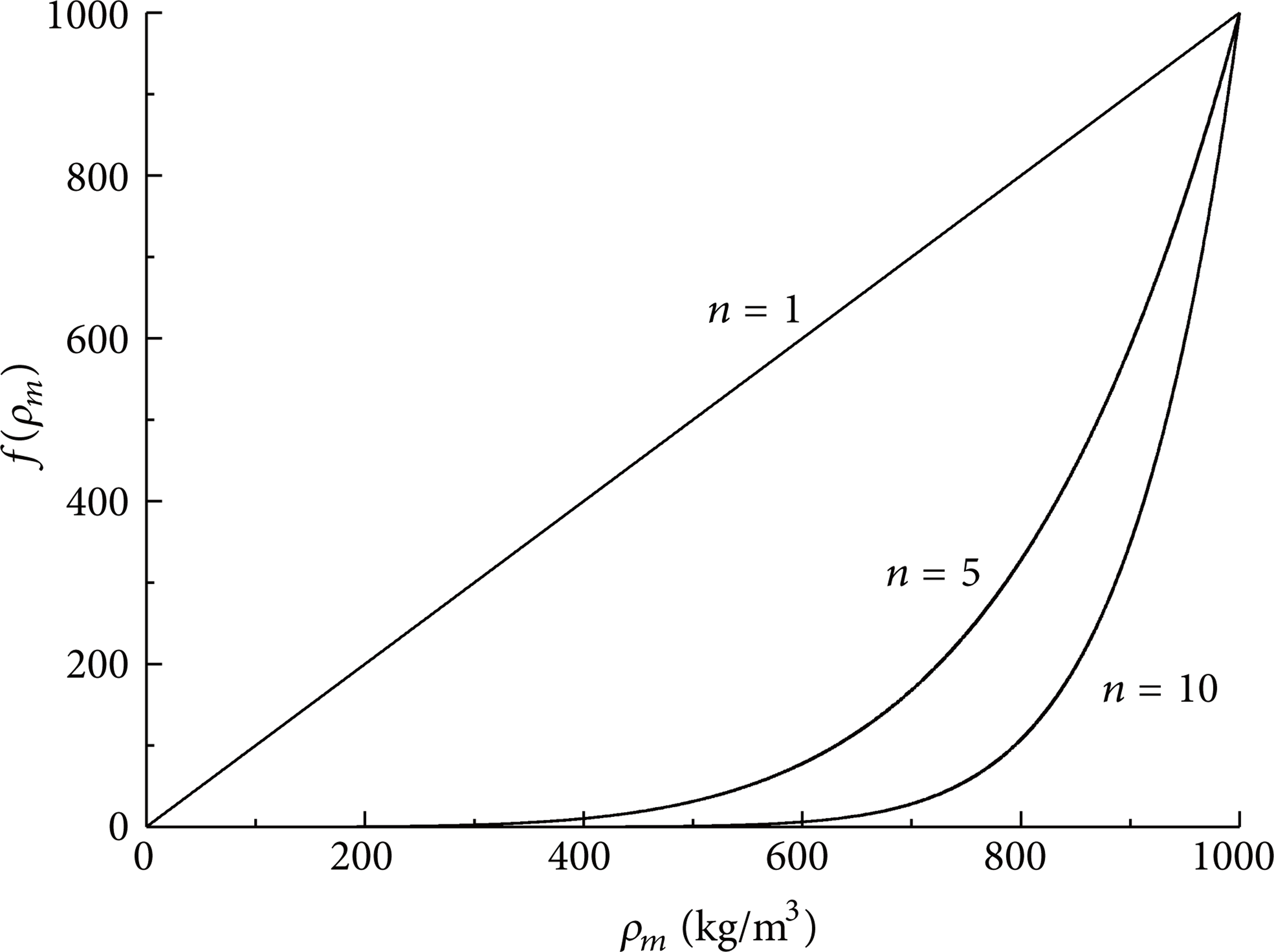
f(ρ_m) ∼ ρ_m.

2.2. Model Francis Turbine

The numerical studies were conducted with a model Francis turbine, whose parameters are listed in Table 1. The computational domain is shown in Figure 3.

Table 1:

Parameters of the model Francis turbine.

Runner diameter D₁ (m)	0.42
Rated head (m)	237
Optimum unit speed n₁₁ (rpm)	67
Optimum unit discharge Q₁₁ (m³/s)	0.38
Number of runner blades Z	17
Number of stay vanes Z_s	24
Number of guide vanes Z₀	24
Relative height of guide vanes $\bar{B_{0}}$	0.18

Figure 3:

Computational domain.

The model gives a 94.54% level of peak efficiency. The performance characteristics determined by model tests under experimental head of 30 m can be seen in Figure 1. Systematic uncertainty on the efficiency measurement of the test rig is less than ±0.25%.

2.3. Computational Details

In order to investigate the validity of the methodology of predicting the incipient and developed inter blade vortex lines of the turbine by cavitation simulations, single-phase flow simulations by RANS RNG k – ∊ turbulence model were also carried out for comparisons. Due to the heavy computational loads, calculations of both cavitating and single-phase flows were performed in steady state.

The model's mesh system was composed of unstructured grids in the spiral case, the stay vanes and the runner, and structured grids in the guide vanes, the draft tube, and the inlet pipe. Commercial software package ICEM was used for mesh discretization. Local refinements to the boundary layer in the runner were applied, to ensure that the values of y⁺ are compatible with the chosen turbulence model (y⁺ < 200 on runner blades). Verification of grid independence was performed with respect to runner efficiency, with total number of grid cells that varied from 2 million to 8 million, as shown in Figure 4. It can be seen that the degree of computational precision is satisfactory when the number of cells is more than 6 million. A mesh with about 7.6 million cells in total was chosen for the simulations. The number of nodes and cells in each part is shown in Table 2.

Table 2:

Number of cells and nodes of each subdomain.

Regions	Inlet pipe	Spiral case and stay vanes	Guide vanes	Runner	Draft tube

Number of nodes	66,625	362,314	176,782	872,047	123,413
Number of cells	62,320	1,837,190	890,278	4,209,796	640,929

Figure 4:

Verification of grid independence.

The three dimensional steady calculations were realized with the MRF (Multiple Reference Frame) model in Ansys CFX. A second-order upwind scheme was used for the discretization of the convective terms, and a second-order centered scheme was used for the source terms. Total pressure, initial values of the turbulent kinetic energy, and turbulent dissipation rate were set at the inlet boundary, while static pressure was set as the outlet boundary condition. For cavitation calculations, cavitation number σ = 0.086 was specified according to the experimental conditions.

3. Results and Discussions

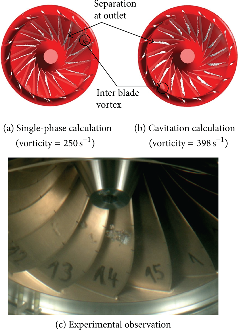
In order to predict the incipient and developed inter blade vortex lines, it is essential to evaluate the compatibility of various vortex identification methods with our simulation cases. A number of vortex identification methods/criteria have been proposed [24], including vorticity criterion, Q criterion, swirling strength criterion, and helicity criterion. By comparing the isosurfaces of the four quantities at corresponding operating points with n₁₁ = 59 r/min and n₁₁ = 72.5 r/min, along the incipient and developed inter blade vortex lines, respectively, it can be concluded that the vorticity criterion is most suitable for distinguishing the vortices. As shown in Figures 5 and 6, distinct differences in the distribution of the isosurfaces of the vorticity can be observed, with vorticity = 250 s⁻¹ with single-phase calculation and vorticity = 398 s⁻¹ with cavitation calculation, between operating conditions along the incipient and developed inter blade vortex lines. Vortices in 2–3 interblade runner flow channels can be seen along the incipient line, and in most flow channels along the developed line.

Figure 5:

Inter blade vortices on the incipient line.

Figure 6:

Inter blade vortices on the developed line.

In order to predict the two vortex lines, seven and nine n₁₁ values were chosen, each with 3∼6 operating conditions for single-phase and cavitation calculations, as shown in Tables 3 and 4, respectively. The incipient and developed inter blade vortex lines were asymptotically derived with vorticity criterion. The results of the predictions with both single-phase and cavitation calculations were compared with experimental observations, as shown in Figure 7. It can be concluded that better agreements were achieved by using the prescribed cavitation calculations. It is also seen that the inflection points on both lines were successfully predicted with cavitation calculations.

Table 3:

Operating conditions for single-phase calculations.

n ₁₁	Q ₁₁
n ₁₁	Incipient			Developed

59	235	230	225	200	190	180
62	250	245	240	230	225	220
63.5	260	250	245	240	235	230
66	265	260	248	230		225
68	265	260	255
70				240	235	230
72.5	260	255	248	240		235

Table 4:

Operating conditions for cavitation calculations.

n ₁₁	Q ₁₁
n ₁₁	Incipient			Developed

59	240	235	230	200	195	190
60	255	250	245	240		225
62	260	255	252	240		235
63.5	270	265	260	250	245	240
65	260	255	250
66	250		245	220	215	210
68	255	250	245
70	250	245	240	230	225	220
72.5	245		240	235		230

Figure 7:

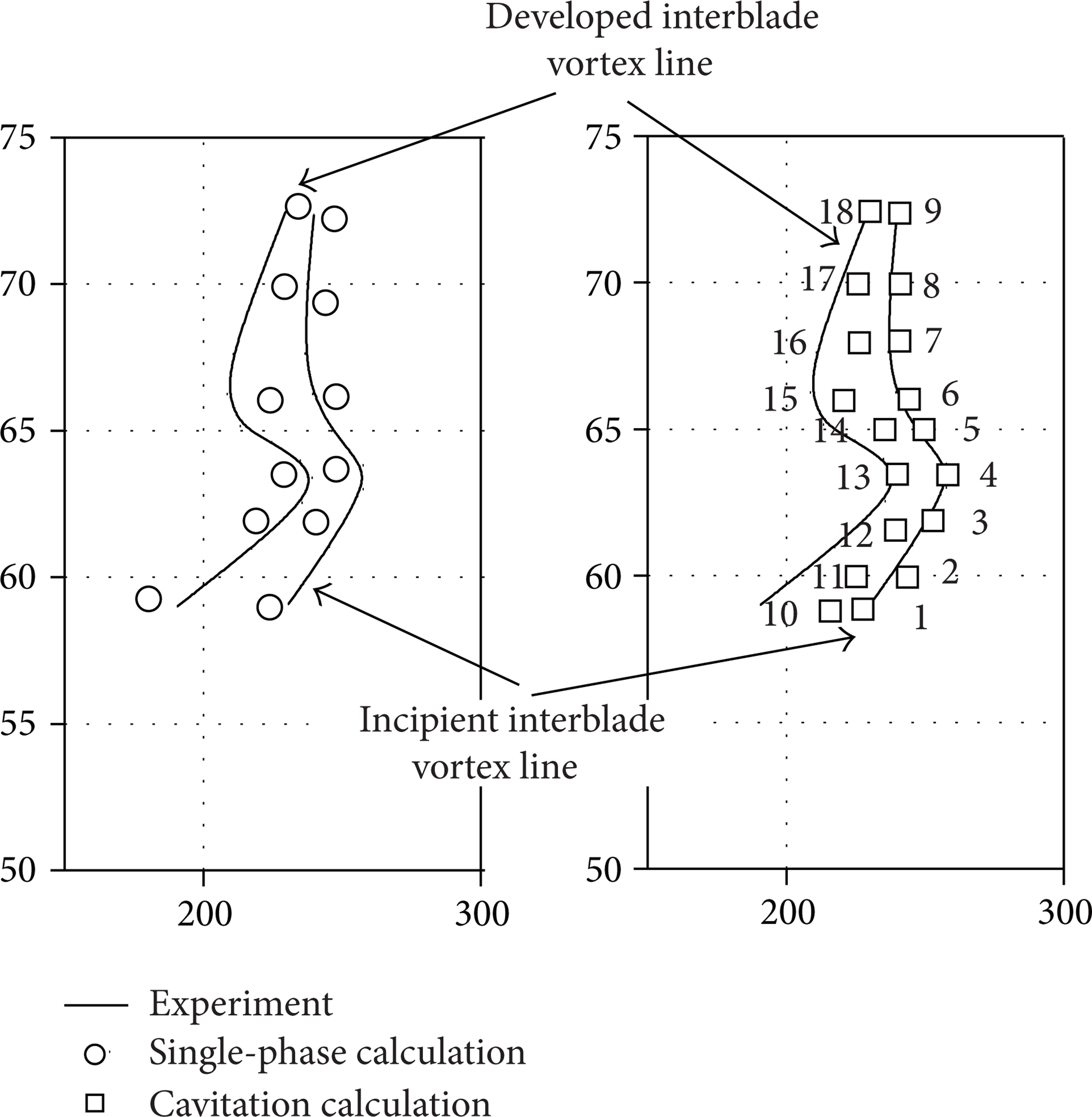
Predictions of the incipient and developed inter blade vortex lines.

Figure 8 shows the velocity triangles at runner inlet, with different operating heads. Higher head corresponds to larger value of absolute velocity c₁, hence smaller n₁₁; lower head corresponds to smaller value of c₁, hence larger n₁₁. The flow angle at optimum n₁₁ is denoted as β₁, which is approximately equal to the blade angle β_b1. The angle of attack i = β₁ – β_b1 ≈ 0 at optimum n₁₁ (no. 7 in Table 5); i > 0 at small n₁₁, where separations on suction sides of the blades occur; i < 0 at large n₁₁, where separations on pressure sides of the blades occur. Bigger angles of attack exist more along the developed inter blade vortex line than incipient line, as shown in Table 5. The existence of the inflection points on the two lines can be roughly explained as below. The occurrence of the inter blade vortices is associated with the variations of the flow angles at runner inlet. This angle tends to be positive with operating conditions at high head, causing flow separations at suction sides of the blades near crown (Figure 9(a)), and it tends to be negative at low head, causing flow separations at pressure sides of the blades near crown (Figure 9(c)). In the case of inflection point (Figure 9(b)), a larger area of separation exists at the crown compared to the case of high head, which induces inter blade vortices at larger Q₁₁.

Table 5:

Angles of attack.

Operating point no.	β_b1 (°)	β₁ (°)	i (°)
1	34.1	78.7	44.7	Incipient inter blade vortex line
3		54.5	20.4
7		34.7	0.6
8		26.9	−7.1
9		21.4	−12.6

10	34.1	84.5	50.5	Developed inter blade vortex line
11		54.7	20.6
13		32.1	−1.9
14		25.6	−8.5
15		20.8	−13.3

Figure 8:

Velocity triangles at runner inlet at different n₁₁ (head).

Figure 9:

Distributions of vorticity on runner.

4. Conclusions

In order to predict the incipient and developed inter blade vortex lines, a method of cavitation calculations was proposed, by solving RANS equations with RNG k – ∊ turbulence model and ZGB cavitation model. Modification of the turbulence viscosity was made to compensate its overestimation in cavitation area. The predictions of a Francis model turbine were derived by an asymptotic approach. By comparing the results with single-phase calculations and experimental observations, it was concluded that the prescribed cavitation calculations could achieve better predictions for the two vortex lines.

Conflict of Interests

The authors declare that there is no conflict of interests regarding the publication of this paper.

Footnotes

Acknowledgments

The authors would like to thank National Natural Science Foundation of China (no. 51076077) and National Science and Technology Ministry of China (ID: 2008BAC48B02) for their financial supports.

References

Huang

Liu

, and Fan

, Research on Prototype Hydro-Turbine Operation, China Electric Power Press, 2010.

Shi

, and Gong

, Noise Reduction in a Low Head Francis Turbine Caused by Runner Inter-Blade Vortices, Dongfang Electric Machinery, 2008.

Grindoz

, Lois de similitudes dans les essays de cavitation des turbines Francis 714. [Ph.D. thesis], EPFL, Lausanne, Switzerland, 1991.

Peng

Chen

, and Jiang

, “Experimental investigation of flow pattern observation and water pressure pulsation per-formed on the three Gorges model turbine,” Water Resources and Hydropower Engineering, vol. 30, no. 11, pp. 8–14, 1999.

Chen

and Peng

, “An experimental study on water pressure fluctuation at Francis turbine runner blade outlet,” Water Resources and Hydropower Engineering, vol. 30, no. 11, pp. 30–32, 1999.

Chen

, and Liu

, “The occurrence and the influence of the interblade vortex on the hydraulic turbine instability,” Large Electric Machine & Hydraulic Turbine, no. 3, pp. 42–46, 2007.

Zhang

Zhu

, and Zhang

, “Numerical investigation on pressure fluctuations induced by interblade vortices in a runner of Francis turbine,” Large Electric Machine & Hydraulic Turbine, no. 6, pp. 35–39, 2009.

Stein

Sick

Doerfler

White

, and Braune

, “Numerical simulation of the cavitating draft tube vortex in a Francis turbine,” in Proceedings of the IAHR 23rd Symposium of Section Hydraulic Machinery, Equipment, and Cavitation, Yokohama, Japan, 2006.

Avellan

, “Introduction to cavitation in hydraulic machinery,” in Proceedings of the 6th International Conference on Hydraulic Machinery and Hydrodynamics, Timisoara, Romania, October 2004.

10.

Kurosawa

Lim

S. M.

, and Enomoto

, “Virtual model test for a francis turbine,” in Proceedings of the 25th IAHR Symposium on Hydraulic Machinery and Systems, vol. 12, Timisoara, Romania, 2010.

11.

Senocak

and Shyy

, “A pressure-based method for turbulent cavitating flow computations,” Journal of Computational Physics, vol. 176, no. 2, pp. 363–383, 2002.

12.

Liu

Dou

H.-S.

, and Zhang

, “Simulations of unsteady cavitating turbulent flow in a Francis turbine using the RANS method and the improved mixture model of two-phase flows,” Engineering with Computers, vol. 27, no. 3, pp. 235–250, 2011.

13.

Merkle

Feng

, and Buelow

, “Computational modeling of the dynamics of sheet cavitation,” in Proceedinogs of the 3rd International Symposium on Cavitation, vol. 4, pp. 307–311, Grenoble, France, 1998.

14.

Kunz

R. F.

Stinebring

D. R.

Chyczewski

T. S.

Boger

D. A.

Gibeling

H. J.

, and Govindan

T. R.

, “Multi-phase CFD analysis of natural and ventilated cavitation about submerged bodies,” in Proceedings of the 3rd ASME/JSME Joint Fluids Engineering Conference (FEDSM '99), FEDSM99–7364, San Francisco, Calif, USA, 1999.

15.

Kunz

R. F.

Boger

D. A.

Stinebring

D. R.

, “A preconditioned Navier-Stokes method for two-phase flows with application to cavitation prediction,” Computers & Fluids, vol. 29, no. 8, pp. 849–875, 2000.

16.

Singhal

A. K.

Athavale

M. M.

, and Jiang

, “Mathematical basis and validation of the full cavitation model,” Journal of Fluids Engineering, vol. 124, no. 3, pp. 617–624, 2002.

17.

Senocak

and Shyy

, “Interfacial dynamics-based modelling of turbulent cavitating flows—part 1: model development and steady-state computations,” International Journal for Numerical Methods in Fluids, vol. 44, no. 9, pp. 975–995, 2004.

18.

Zwart

Gerber

, and Belamri

, “A two-phase flow model for predicting cavitation dynamics,” in Proceedings of the 5th International Conference on Multiphase Flow, Paper No.152, Yokohama, Japan, 2004.

19.

Zwart

, “Numerical modelling of free surface and cavitating flows,” in Proceedings of the Industrial Two-Phase Flow (CFD '05), VKI Lecture Series, pp. 1–25, Von Karman Institute for Fluid Mechanics, Brussels, Belgium, May 2005.

20.

Yin

Wang

, and Walters

, “A modified model for computation of flows with large streamline curvature,” Advances in Mechanical Engineering, vol. 2013, Article ID 59242, 10 pages, 2013.

21.

Coutier-Delgosha

Reboud

J. L.

, and Delannoy

, “Numerical simulation of the unsteady behaviour of cavitating flows,” International Journal for Numerical Methods in Fluids, vol. 42, no. 5, pp. 527–548, 2003.

22.

Coutier-Delgosha

Fortes-Patella

, and Reboud

J. L.

, “Evaluation of the turbulence model influence on the numerical simulations of unsteady cavitation,” Journal of Fluids Engineering, vol. 125, no. 1, pp. 38–45, 2003.

23.

Coutier-Delgosha

Reboud

, and Albano

, “Numerical simulation of the unsteady cavitation behavior of an inducer blade cascade,” in Proceedings of the ASME Fluids Engineering Division Summer Meeting (FEDSM '00), ASME, New York, NY, USA, 2000.

24.

Jiang

Machiraju

, and Thompson

, Detection and Visualization of Vortices, Visualization Handbook, Academic Press, 2004.

Numerical Predictions of the Incipient and Developed Interblade Vortex Lines of a Model Francis Turbine by Cavitation Calculations

Abstract

1. Introduction

2. Numerical Methods

2.1. Cavitation Simulation

2.2. Model Francis Turbine

2.3. Computational Details

3. Results and Discussions

4. Conclusions

Conflict of Interests

Footnotes

Acknowledgments

References